Tutorial: Building an Inline Holographic Microscope
In this workshop, we will construct an inline holographic microscope using the UC2 modular microscope toolbox. Inline holography is a lensless imaging technique that uses coherent light interference to capture and reconstruct 3D images of transparent samples. This experiment demonstrates fundamental principles of wave optics, Fresnel diffraction, and digital image reconstruction while providing hands-on experience with modern computational imaging techniques.
Materials Needed
Optical Components:
- LED light source (preferably white LED for broad spectrum)
- Gel color filter (green or red) for quasi-monochromatic illumination
- Aluminum foil or thin metal sheet for pinhole creation
- Precision pinhole (10-50 μm diameter) or needle for custom pinhole
- Transparent samples (biological specimens, microstructures, dust particles)
Detection Equipment:
- ESP32 camera module with wide-angle lens
- Computer with WiFi capability for wireless image capture
- Optional: Higher resolution camera (HIKrobot or similar) for advanced applications
Mechanical Components:
- UC2 modular microscope toolbox (minimum 4 cubes)
- LED holder insert for UC2 cube
- Sample holder for transparent specimens
- Base plates for system stability
- Puzzle pieces for cube connections
Software and Analysis:
- Jupyter notebook environment
- Python libraries: NumPy, Matplotlib, SciPy
- OpenUC2 holographic reconstruction code
- ImSwitch software (optional for real-time processing)
Safety and Environment:
- Dark or controlled lighting environment
- Stable surface for vibration isolation
- Proper sample handling equipment
TODO: Add specific LED wavelength recommendations and optimal power levels TODO: Include computer system requirements for real-time reconstruction
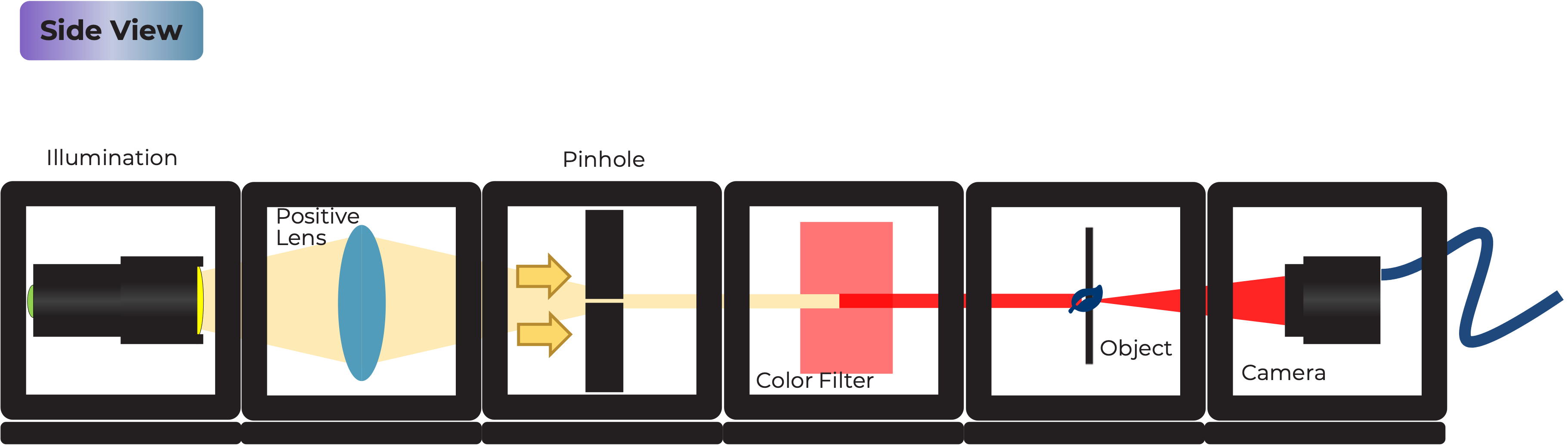
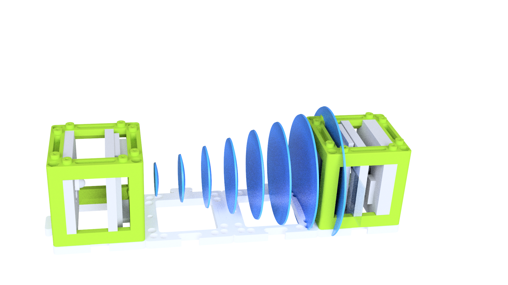
Diagram
Schematic diagram showing the inline holographic microscope layout with LED source, pinhole, sample, and detector
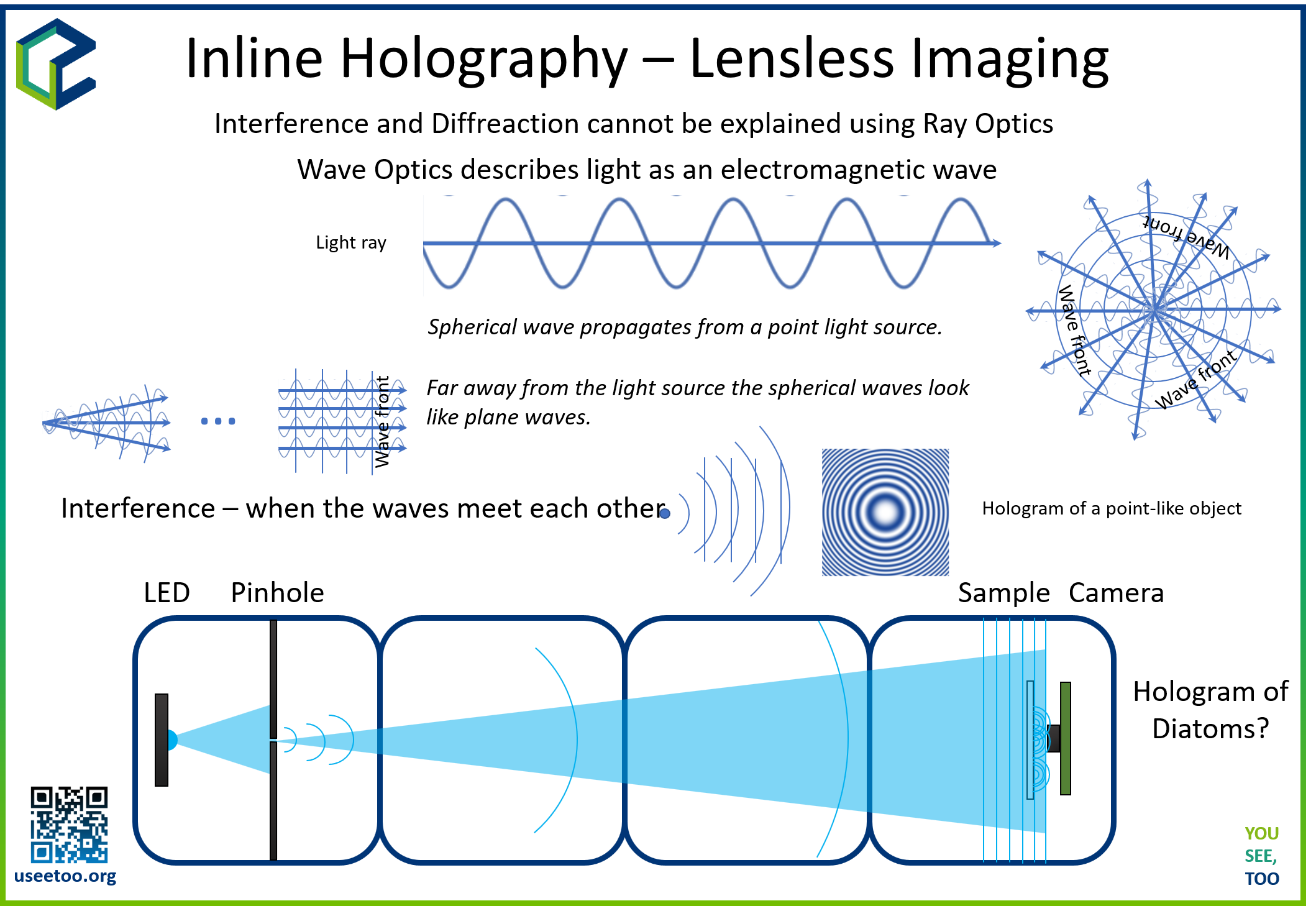
Theory of Operation
The inline holographic microscope operates as a lensless imaging system where coherent light from a point source illuminates a transparent sample. The scattered light from the sample interferes with the unscattered reference beam directly on the detector surface, creating a holographic interference pattern. This pattern contains both amplitude and phase information about the sample, which can be computationally reconstructed to visualize the original object.
Unlike conventional microscopy that uses lenses to form images, holographic microscopy relies on digital reconstruction algorithms to focus and refocus images at different distances. This approach offers several advantages: large field of view, no optical aberrations, and the ability to focus on different depth planes post-acquisition.
Theoretical Background
Holography Principles
Holography is based on the recording and reconstruction of light wave interference patterns. In inline holography, three key wave components interact:
- Reference Wave: Unperturbed light passing through empty space
- Object Wave: Light scattered by the sample
- Interference Pattern: Superposition of reference and object waves
Fresnel Diffraction and Propagation
The propagation of light from the sample to the detector follows Fresnel diffraction theory. The complex amplitude at the detector plane is given by:
U(x,y,z) = -i/(λz) ∬ U(x',y',0) exp[ik/(2z)((x-x')² + (y-y')²)] dx'dy'
Where λ is the wavelength, z is the propagation distance, and k = 2π/λ is the wave number.
Digital Reconstruction
The reconstruction process involves numerically propagating the recorded intensity pattern back to the sample plane using the Fresnel-Kirchhoff diffraction integral. This is efficiently implemented using Fast Fourier Transform (FFT) algorithms:
- Forward FFT: Convert intensity pattern to frequency domain
- Phase Correction: Apply propagation phase factor
- Inverse FFT: Transform back to spatial domain
The propagation phase factor is: H(fx,fy,z) = exp[ikz√(1 - λ²fx² - λ²fy²)]
Limitations and Challenges
Inline holography faces several fundamental limitations:
- Twin Image Problem: Loss of phase information creates overlapping virtual images
- Limited Resolution: Bounded by pixel size and numerical aperture
- Sparse Sample Requirement: Dense samples create complex interference patterns
- Coherence Requirements: Spatial and temporal coherence affect image quality
Modern Applications
Inline holography has found applications in:
- Medical diagnostics: Blood cell analysis, malaria detection
- Environmental monitoring: Plankton and microorganism studies
- Industrial inspection: Particle size and distribution analysis
- Materials science: Thin film characterization
- Astronomical imaging: Space-based telescopy applications
TODO: Add mathematical derivations for advanced students TODO: Include specific resolution calculations for different system parameters
Tutorial: Inline Holographic Microscope Setup
Complete assembly showing all components needed for the inline holographic microscope
Step 1: Assemble the Optical Components
SAFETY INSTRUCTIONS
⚠️ GENERAL SAFETY WARNINGS:
- Handle optical components carefully to avoid scratches and contamination
- Work in controlled lighting conditions to minimize background interference
- Use proper sample handling techniques to prevent contamination
- Ensure stable mounting to prevent component movement during measurements
- Keep work area clean and organized to avoid losing small components
1.1: Prepare the Illumination Source
Create a quasi-coherent point source by:
- Insert LED into the UC2 LED holder
- Place gel color filter in front of LED (green or red recommended)
- Create a small pinhole (10-50 μm) in aluminum foil using a fine needle
- Mount the pinhole-filter assembly in the UC2 cube
Note: The pinhole size determines spatial coherence - smaller pinholes provide better coherence but reduced brightness.
1.2: Build the Base Configuration
Assemble the system with four UC2 cubes in a linear arrangement:
- Cube 1: LED source with pinhole
- Cube 2: Empty spacer cube
- Cube 3: Sample holder cube
- Cube 4: Camera detector cube
Connect all cubes with base plates for mechanical stability.
1.3: Position the Sample
Mount your transparent sample as close as possible to the camera sensor:
- Use minimal sample thickness (coverslip or thin film)
- Ensure sample is sparse (isolated particles work best)
- Avoid dense or thick samples that create complex scattering
1.4: Optimize Source-Sample-Detector Geometry
The key distances are:
- Source-to-sample distance (L1): 10-20 cm for good illumination uniformity
- Sample-to-detector distance (L2): <5 mm for high resolution
- Magnification ratio: M = L1/L2 (typically 20-100x)
TODO: Add specific distance calculations for different magnification requirements
Step 2: Electronics
2.1: ESP32 Camera Setup
- Connect ESP32 camera module to power supply
- Configure WiFi connection for wireless image capture
- Test camera functionality with basic image acquisition
- Adjust exposure and gain settings for optimal signal-to-noise ratio
2.2: Camera Software Configuration
- Connect to ESP32 web interface via WiFi
- Set image resolution (typically VGA or higher)
- Adjust compression settings (minimize JPEG artifacts)
- Test image capture and download functionality
TODO: Add specific firmware versions and configuration parameters
Step 3: Alignment and Optimization
3.1: System Alignment
- Turn on LED source and observe illumination pattern
- Check for uniform illumination across the field of view
- Ensure pinhole is properly centered and clean
- Verify camera is recording the sample area
3.2: Environmental Optimization
- Eliminate stray light: Cover system with dark enclosure
- Minimize vibrations: Use stable surface or isolation table
- Control air currents: Avoid drafts that can cause intensity fluctuations
- Thermal stability: Allow system to reach thermal equilibrium
3.3: Sample Optimization
Test with different samples to find optimal conditions:
- Start with sparse dust particles or pollen
- Progress to biological samples (cells, bacteria)
- Avoid thick or dense samples initially
Step 4: Digital Reconstruction (ImSwitch Integration)
4.1: Basic Python Reconstruction
import numpy as np
import matplotlib.pyplot as plt
from scipy.fft import fft2, ifft2

def reconstruct_inline_hologram(hologram, wavelength, pixel_size, distance):
    """
    Reconstruct inline hologram using Fresnel propagation

    Parameters:
    hologram: 2D numpy array of intensity values
    wavelength: light wavelength in meters
    pixel_size: detector pixel size in meters
    distance: reconstruction distance in meters
    """
    # Get image dimensions
    ny, nx = hologram.shape

    # Create frequency coordinates
    fx = np.fft.fftfreq(nx, pixel_size)
    fy = np.fft.fftfreq(ny, pixel_size)
    FX, FY = np.meshgrid(fx, fy)

    # Calculate propagation phase factor
    k = 2 * np.pi / wavelength
    phase_factor = np.exp(1j * k * distance * np.sqrt(1 - (wavelength * FX)**2 - (wavelength * FY)**2))

    # Apply Fresnel propagation
    hologram_fft = fft2(hologram)
    reconstructed_fft = hologram_fft * phase_factor
    reconstructed = ifft2(reconstructed_fft)

    return reconstructed

# Example usage
wavelength = 532e-9  # Green light wavelength
pixel_size = 2.4e-6  # Typical camera pixel size
distance = -0.01     # Reconstruction distance (negative for refocusing)

# Load and process hologram
img = plt.imread("hologram.png")
reconstructed = reconstruct_inline_hologram(img, wavelength, pixel_size, distance)

# Display results
plt.figure(figsize=(12, 4))
plt.subplot(1, 3, 1)
plt.imshow(img, cmap='gray')
plt.title('Original Hologram')
plt.subplot(1, 3, 2)
plt.imshow(np.abs(reconstructed), cmap='gray')
plt.title('Reconstructed Amplitude')
plt.subplot(1, 3, 3)
plt.imshow(np.angle(reconstructed), cmap='hsv')
plt.title('Reconstructed Phase')
plt.show()
4.2: ImSwitch Integration
For real-time reconstruction:
- Install ImSwitch software with holography plugins
- Configure camera connection in ImSwitch
- Set reconstruction parameters (wavelength, distances)
- Enable real-time processing for live focusing
4.3: Advanced Processing
Implement additional processing steps:
- Background subtraction: Remove illumination variations
- Noise filtering: Apply appropriate image filters
- Multi-distance reconstruction: Focus stacking for extended depth
- Phase unwrapping: Extract quantitative phase information
TODO: Add specific ImSwitch configuration files and parameters
Experiment 1: Basic Hologram Recording and Reconstruction
1.1: Capture Reference Holograms
- Start with no sample to establish background
- Record intensity pattern from pure illumination
- Note any interference fringes or artifacts
- Save reference image for background subtraction
1.2: Sample Hologram Acquisition
- Insert sparse sample (dust, pollen, or cells)
- Capture hologram showing interference fringes
- Verify sufficient contrast and fringe visibility
- Record multiple images at different positions
1.3: Basic Reconstruction
- Load hologram image into reconstruction software
- Set appropriate wavelength and distance parameters
- Perform reconstruction at the sample plane
- Compare with direct sample observation
Experiment 2: Multi-Distance Reconstruction
2.1: Focus Stacking
- Reconstruct at multiple distances around the sample plane
- Create focus stack to visualize 3D structure
- Identify optimal focus distance for each sample feature
- Generate extended depth-of-field image
2.2: 3D Visualization
- Map focused features at different depths
- Create 3D representation of sample structure
- Measure feature positions and sizes
- Compare with theoretical expectations
2.3: Resolution Analysis
- Measure resolution using known test samples
- Compare with theoretical resolution limits
- Identify factors limiting resolution
- Optimize system parameters for best performance
Experiment 3: Quantitative Analysis
3.1: Phase Imaging
- Extract phase information from complex reconstruction
- Unwrap phase data to obtain continuous values
- Convert phase to optical path differences
- Measure sample thickness or refractive index
3.2: Particle Analysis
- Use automated detection algorithms
- Measure particle sizes and positions
- Analyze size distributions
- Track particle motion (if applicable)
3.3: Comparative Studies
- Compare holographic and conventional microscopy
- Analyze advantages and limitations
- Determine optimal sample types and conditions
- Document measurement accuracy and precision
Safety Guidelines and Best Practices
General Laboratory Safety
- Clean optical surfaces carefully using appropriate lens tissues and solutions
- Handle samples properly to avoid contamination
- Store equipment safely when not in use
- Document all experimental parameters for reproducibility
Data Management
- Save raw holograms in uncompressed formats when possible
- Record all experimental parameters (distances, wavelengths, settings)
- Back up important data regularly
- Document reconstruction parameters for future reference
TODO: Add specific safety protocols for biological samples
Troubleshooting Guide
Common Problems and Solutions
Problem: No Interference Fringes Visible
Possible Causes:
- Insufficient coherence
- Poor pinhole quality
- Excessive background light
- Wrong sample-detector distance
Solutions:
- Check pinhole size and quality
- Improve light source coherence
- Better environmental light control
- Adjust geometric parameters
Problem: Poor Reconstruction Quality
Possible Causes:
- Incorrect reconstruction parameters
- JPEG compression artifacts
- Twin image interference
- Phase retrieval errors
Solutions:
- Verify wavelength and distance values
- Use uncompressed image formats
- Apply twin image suppression algorithms
- Improve phase reconstruction methods
Problem: Low Image Contrast
Possible Causes:
- Dense sample scattering
- Improper illumination
- Background interference
- Camera settings
Solutions:
- Use sparser samples
- Optimize illumination uniformity
- Implement background subtraction
- Adjust camera exposure and gain
Problem: Unstable Results
Possible Causes:
- Environmental vibrations
- Temperature fluctuations
- Air current interference
- Mechanical instability
Solutions:
- Improve vibration isolation
- Control environmental conditions
- Enclose optical system
- Secure all mechanical connections
TODO: Add troubleshooting for specific software issues
Assessment Questions
Conceptual Understanding
Holography Principles:
- Explain the difference between inline and off-axis holography
- Describe how phase information is encoded in interference patterns
- Why is coherent illumination essential for holographic imaging?
Digital Reconstruction:
- Describe the role of FFT in holographic reconstruction
- Explain the twin image problem and potential solutions
- How does reconstruction distance affect image focus?
System Design:
- Compare advantages and disadvantages with conventional microscopy
- What factors limit the resolution of inline holography?
- How would you optimize the system for different sample types?
Problem-Solving Exercises
Parameter Optimization:
- Calculate optimal pinhole size for given source-sample distance
- Determine reconstruction distance for best focus
- Estimate theoretical resolution for your system
Application Design:
- Design modifications for flowing sample analysis
- Adapt system for different wavelength operation
- Integrate with automated sample handling
Extension Projects
Advanced Techniques:
- Implement machine learning for artifact removal
- Develop real-time processing algorithms
- Explore multi-wavelength holography
Research Applications:
- Apply to biological sample analysis
- Study dynamic processes in microfluidics
- Investigate materials characterization applications
TODO: Add specific calculation examples and expected results TODO: Include links to current research and applications
Resources and References
Historical Context
- Dennis Gabor (1948): Invented holography, Nobel Prize 1971
- Fresnel and Kirchhoff: Diffraction theory foundations
- Digital holography development: 1990s computational advances
Modern Applications
- Medical diagnostics: Point-of-care blood analysis
- Environmental monitoring: Plankton studies and water quality
- Industrial inspection: Quality control and defect detection
- Space applications: Compact imaging systems for satellites
Further Reading
- Principles of Optics - Born & Wolf
- Digital Holography and Digital Image Processing - Schnars & Jüptner
- Current research papers in Applied Optics and Optics Letters
TODO: Add specific links to current research papers and applications TODO: Include bibliography of recommended textbooks and resources
Known Limitations and Future Improvements
Current Limitations:
- Twin image artifacts in reconstruction
- Limited resolution compared to conventional microscopy
- Requirement for sparse samples
- Sensitivity to environmental disturbances
Potential Improvements:
- Machine learning artifact removal
- Advanced phase retrieval algorithms
- Multi-wavelength techniques
- Improved vibration isolation
TODO: Add development roadmap for system improvements
Creating the Light Source The holographic microscope begins with a specially prepared light source. An LED, filtered through a gel color filter and focused through a pinhole in aluminum foil, generates quasi-monochromatic coherent light. This coherent light source is essential for the interference patterns necessary for holography.
Sample and Camera Setup A transparent sample is placed in the path of the coherent light source. As the light passes through the sample, it becomes scattered, creating a complex wavefront. The camera, integrated into the same cube as the sample holder, captures this scattered light as an interference pattern, known as the hologram.
Fresnel Propagation When the scattered light reaches the camera sensor, it captures the intensity of the interference pattern. In inline holography, both the object and reference beams travel along the same path to the sensor, causing them to interfere. The Fresnel propagation is used to numerically propagate the hologram from the sensor plane to the object plane and vice versa.
Fresnel propagation is a mathematical process that simulates the propagation of light waves between two planes. It utilizes the Fresnel-Kirchhoff diffraction integral to calculate the complex wavefront at a given distance from the hologram plane. This numerical transformation involves the Fast Fourier Transform (FFT), which efficiently converts the hologram from spatial to frequency coordinates.
Fast Fourier Transform (FFT) The FFT is a powerful algorithm used to compute the discrete Fourier transform of an image. It efficiently calculates the frequency components present in an image, providing valuable information about its structure. In our holographic microscope, the FFT is used to transform the captured hologram from real space to frequency space.
The transformed hologram in frequency space contains complex information about the sample's phase and amplitude. However, due to the lensless nature of the microscope, the phase information is lost during the hologram capture process. As a result, additional artifacts, such as the twin-image and ringing artifacts, can occur during hologram reconstruction.
Assembly Steps
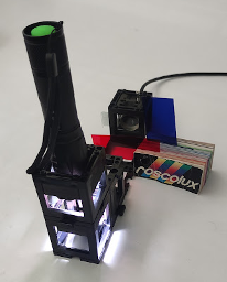
Creating the Light Source
- Attach the LED holder to one side of a cube using the provided puzzle pieces.
- Insert the LED into the holder and connect it to an appropriate power source or use the battery-driven one without external power.
- Produce a pinhole using aluminium foil: Take a needle, fold the aluminium foil 8 times, punch a hole, unfold the foil and take the smallest hole that is still intact
- Position the aluminum foil with a pinhole in front of the LED-light source, allowing the light to pass through the pinhole
- Place the gel color filter in front of the aluminium foil to create a quasi-monochromatic coherent light source. .
Setting Up the Sample and Camera
- Place an empty cube right next to the light source cube.
- Position another empty cube on the other side of the light source cube.
- Combine the transparent sample mount and the camera module into a single cube. Mount the sample onto the camera sensor surface, ensuring that there is little space between them.
Assembling the Microscope
- Arrange the cubes in the following order (from left to right): Light Source Cube, Empty Cube, Empty Cube, Sample & Camera Cube.
- Securely mount each cube on puzzle pieces at the lower end and upper bar using the puzzle pieces to ensure stability.
Powering Up the Microscope
- Use the ESP32 camera inside the cube and flash the XIAO firmware
- The link comes here: https://matchboxscope.github.io/firmware/FLASH.html
- Turn on the camera and connect to it via Wi-Fi (the Wifi SSID is Matchboxscope-****, where the number is displayed during boot-up phase in the serial monitor after the flashing process) using a web app or browser (http://192.168.4.1)
- Power on the LED light source.
Adjusting the Contrast
- Check the camera's output for the captured image.
- If the contrast is low due to scattering background light, cover the system with a box or use some shading to prevent direct light from hitting the sensor.
Reconstructing the Hologram
- Capture an image using the ESP32 camera and download it onto your computer (full resolution, i.e. 1600x1200, the capture button in the GUI will offer to download the image, give it some name and save it).
- Start the Jupiter notebook server in the command line.
- (Installation:
pip install jupyterlaband then start it usingjupyterlab) - Create a new Jupiter notebook for hologram reconstruction (see step 7)
- Input the path to the downloaded image file in the notebook.
- Reconstruct the hologram using a fast Fourier transform (FFT) and numerical back-propagation.
- Be aware of twin-image artifacts and potential ringing artifacts in the reconstruction due to interference.
Create a Jupyter notebook and reconstruct the images
The following code will help you go through the process. Create a new Jupyter Notebook, change the path to the file and try it out.
# Import necessary libraries
from io import BytesIO
import matplotlib.pyplot as plt
import numpy as np

# Define a function to reconstruct inline hologram
def reconstruct_inline_hologram(hologram, wavelength, ps, distance):
    # Inverse space
    Nx = hologram.shape[1]  # Number of columns in the hologram
    Ny = hologram.shape[0]  # Number of rows in the hologram
    fx = np.linspace(-(Nx-1)/2*(1/(Nx*ps)), (Nx-1)/2*(1/(ps*Nx)), Nx)
    fy = np.linspace(-(Ny-1)/2*(1/(ps*Ny)), (Ny-1)/2*(1/(ps*Ny)), Ny)
    Fx, Fy = np.meshgrid(fx, fy)

    # Calculate the kernel using the wavelength and distance
    kernel = np.exp(1j * (2 * np.pi / wavelength) * distance) * np.exp(1j * np.pi * wavelength * distance * (Fx**2 + Fy**2))

    # Compute the centered FFT of the hologram
    E0fft = np.fft.fftshift(np.fft.fft2(hologram))

    # Multiply the spectrum with the Fresnel phase factor
    G = kernel * E0fft
    Ef = np.fft.ifft2(np.fft.ifftshift(G))

    # Return the absolute value of the reconstructed hologram
    return np.abs(Ef)

# Define an asynchronous function to process the image and reconstruct the hologram
async def process(img, distance=0.007, wavelength=450e-9, pixelsize=5e-6):
    img = np.array(img)
    holo = reconstruct_inline_hologram(img, wavelength=wavelength, ps=pixelsize, distance=distance)
    return holo

# Main function that can be used to continuously process images (currently empty loop)
def main():
    while True:
        # Properly call the process function with required parameters
        pass  # Here, you should include the logic to process the images as required

# Read an image
img = plt.imread("/PATH/TO/IMAGE/image.png")
# Process the red channel (index 2) of the image to reconstruct the hologram
holo = await process(img[:,:,2])
# Display the reconstructed hologram
plt.imshow(np.abs(holo))
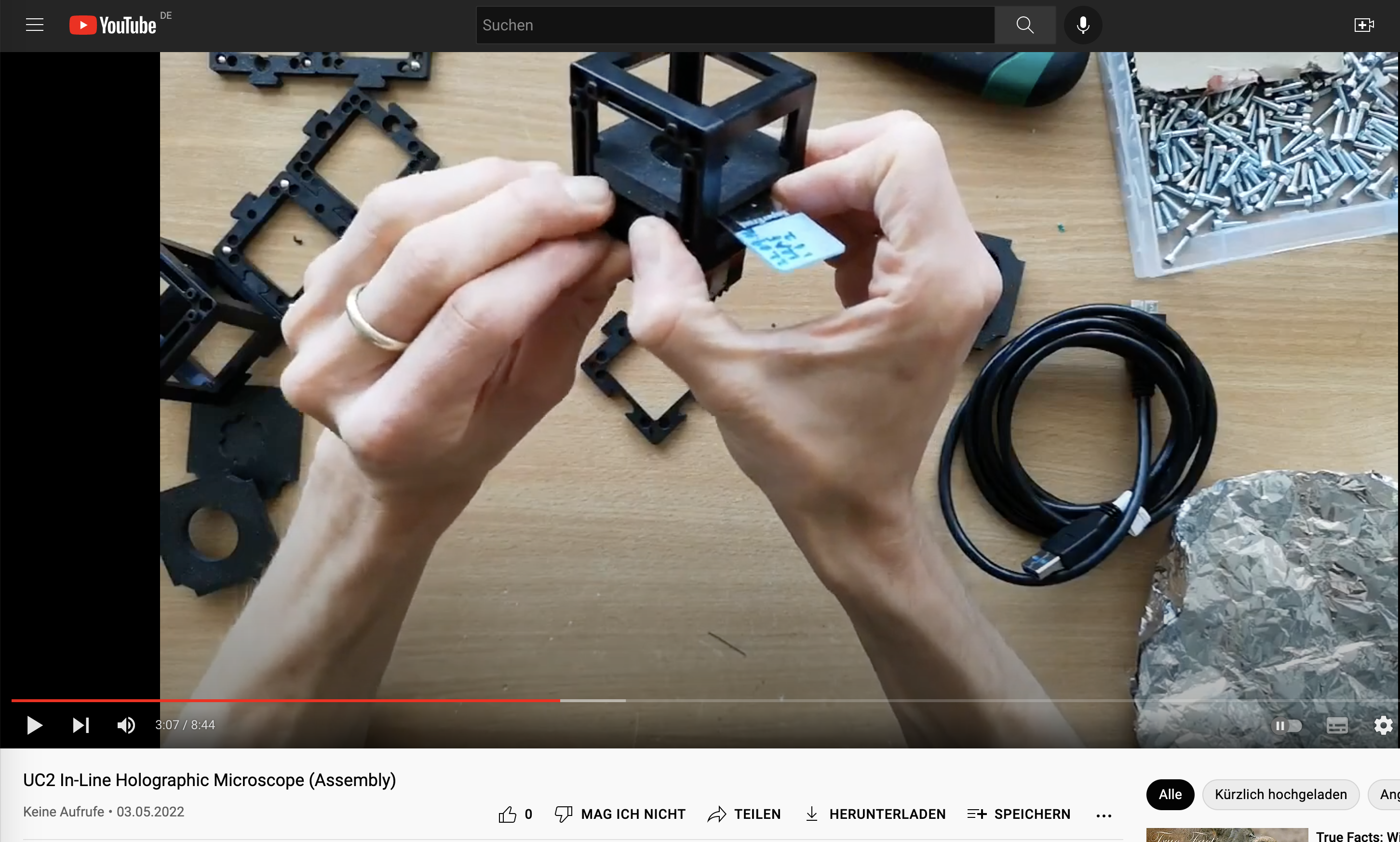
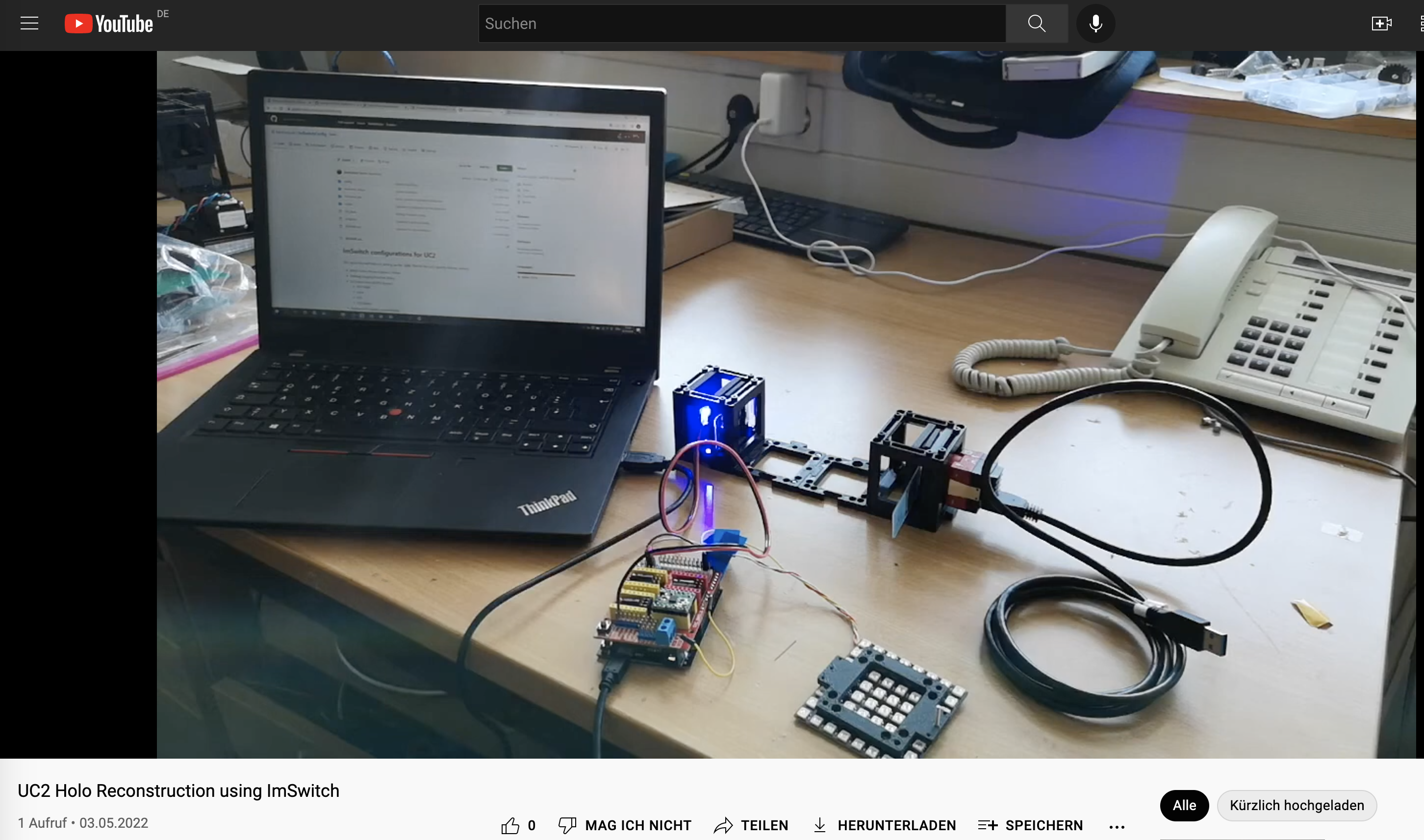
Assembly Video
In this video you will learn how to setup a UC2 system and also how to build the holographic Microscope
Conclusion
Congratulations! You have successfully built an inline holographic microscope using the UC2 modular microscope toolbox. This simple yet powerful setup allows you to observe transparent samples and explore the fascinating world of holography and coherent light sources. By understanding the principles of Fresnel propagation and Fast Fourier Transform, you can reconstruct digital holograms and visualize 3D structures in your samples. Have fun experimenting with different samples and refining your holographic imaging techniques!
Known Problems
- distance between sensor/sample
- stray Light
- sample not sparse enough
Very Experimental: Reconstruct Holograms with ImSwitch
Prerequirements Here you will finde a guide how to setup the ImSwitch Software:
- Download the Software package from Dropbox
- Install Anaconda (Important: When you're asked to add Anaconda to the
PATHenvironment, sayYES!) - Install Arduino + all drivers
- Install the CH340 driver
- Extract
ImSwitch.zipto/User/$USER$/Documents/ImSwitch(clone or download from GitHub) - Extract
ImSwitchConfig.zipto/User/$USER$/Documents/ImSwitchConfig(clone or download from GitHub) - Optional: Install Visual Studio Code + the Python plugin => setup the Visual studio code IDE for Python
Install ImSwitch for UC2
- Open the anaconda command (Windows + R => "CMD" => enter)
- Type:
conda create -n imswitch - Wait until environment is created
- Type:
conda activate imswitch - Type:
cd /User/$USER$/Documents/ImSwitch - Type:
pip intall -r requirements.txt - Type:
pip intall -e ./ - Type:
imswitch
Reconstruction
This video will show you how to reconstruct holographic data using UC2 and ImSwitch.
Things to explore:
- Get Familiar with ImSwitch
- Get a sparse sample e.g. plankton on coverslip would be best, or just dust/sand/cheeck cells and try to acquire some holograms
Refocusing using ImSwitch
Using the In-line Holography plug-in widget in ImSwitch we can refocus the sample by using a propagator in reverse from the recorded hologram in real-time.
The In-line holography experiment can also be produced with a laser source. In this version of the In-line holography setup, we use white light as source and we use filters to have quasi-monochromatic light illuminating the sample.
ADDITIONAL Speach-to-text
The first experiment will be the inline holographic microscope. This is a relatively simple experiment where we can show both the temporal and especially coherence. We will create a lensless microscope where we use an LED that is filtered by a color filter and pinhole to create a quasi one of chromatic coherent light source. This is then illuminating the transparent sample that is sparse before the scattered wave is sitting the camera sensor. This is relatively simple to build with the C2 system; for this, we only need the LED holder, a gel color filter, as it sees from theaters, aluminum foil where we'll stitch in a hole in order to create a local pinhole, some space between this created light source and the sample, and then the sample that this ultimately glued onto the sensor very closely so that the pinhole virtually scales in size as the ratio between the distance of the light source to the sample and sample to the sensor. In order to build the system, we will place the here created light source on the far left; then another empty cube follows right next to it; then another empty cube follows on the right-hand side; and then we combine the sample mount and the camera into one cube so that the distance between the sample and the camera is minimized. All these cubes should be mounted on puzzle pieces on the lower end and the upper bar so that the whole system becomes stable. We will turn on the camera and also turn on the lights source. Then we go to the web app after connecting to the camera through Wi-Fi, and then we will try to see any variation in the contrast of the camera. If the contrast is not high enough because of this scattering background light, we have to cover the system with a box or with some closing so that there's no straight lights hitting the sensor. This will make a very bad result in the reconstruction. When you're lucky, you can see the sample as a kind of shadow on the sensor already. The core idea now is to reconstruct this digital hologram, where we have to carefully maximize the quality of the file image. Compression artifacts from the ESP32 camera are unavoidable and will eventually degrade the final image results. What we are going to do now is to temper in image and then back propagate the distance from the sensor to the sandal plane using a numerical transformation. What this really means is that we take the image and take every pixel and back propagated by a certain distance numerically. This is done using a fast-year transform where we first fiatransform the image so that it is in frequency space; then we multiply it with a parabolic face Factor, and then we inverse full-year transform the results to end up in real space again. This becomes a convolution of the Fresnel colonel, which essentially propagates every pixel edge of certain distance depending on the wavelength and sampling rate. We can conveniently do that in Python with the Script that is provided by the Jupiter notebook. For this, we go to the website of the ESP32, hit the capture button, and download the image onto the computer. Then we start the Jupiter notebook server by opening the command line in Windows or in Linux and enter Jupiter notebook. Then we go to the browser and open the example Jupiter notebook that will reconstruct our hologram. We will enter the path of our downloaded image file and then reconstruct the results. There are several problems which we can describe but not solve at the moment for stop inland holography, as the name already says, has the problem that the light source and the scattered wave interfere in line. That means the point source will create spherical waves that are propagating its free space and will become almost a plain wave when it's the sample. Here some parts of the wave are scattered where which means that a plane wave is altered in its face depending on the face of the microscopic example, and some portion of the wave is an altered. That means after the sample the unchecked and scattered wave are propagating to the sensor where the two amplitudes are superposing. That means they add up for stuff since our camera detector cannot record amplitudes since the object of frequency is very very high. We are averaging out over time. That means that we will record intensity values in the end. This also means that the information about the face is getting lost. When we are reconstructing the hologram, the color will differentiate whether the sample is before or behind the sensor since the face information is that anymore. This means that in the reconstruction, the so-called twin image always overlays the real image in the end. This causes an avoidable ringing artifacts in the reconstruction. There are some ways to remove it, for example by estimating the face using iterative algorithms or model-based approaches, where we take the full image acquisition process into account. Alternatively, suit also be machine learning algorithms where an algorithm estimates the background and remove these artifacts. However, here we won't use these algorithms as we just want to learn how we can reconstruct the simple.
Some notes on the transform that we have just used here. Briefly, it is a transformation from spatial to frequency coordinates. This sounds very abstract, but for example, our ear does this all the time. When we talk, our voice generates a vibration of the air. That means different frequencies are oscillating and add up to something like noise. Our ear, in turn, has the cochlear where many nerve cells, in turn, are oscillating depending on the resonance frequency of every cell. In a way, they are unmixing the noise and modulate the different frequencies. That means that if you're singing like an A, there is the fundamental frequency and several higher and lower harmonics. And lens does something very similar but in two dimensions. You can have optical frequencies where, for example, a grating that is having stripes that represent on and off and on and off
at a certain distance represent periodic structure. It lens when you place something in the focal plane will then flea transform this into the demodulated frequency components. When you, for example, have a periodic structure like a grating, it will produce two pieces in its Fourier transform or in its focal length on the object side. A fast Fourier transform is its equivalent in the computational science. You can take an image and then represent it in its frequency components for stock that means it tries to estimate the sum of all the different frequency components that make up the image. We use this fast Fourier transform in our code to bring it from real space to frequency space and back again. But since we start with an image without an amplitude or without the face, lack the information.
This property creates additional artifacts since relax the information of the face when we record intensity values on our camera, we also limited to samples that I see like just for the tomt capture in the watcher. The optical resolution of our microscope is bound to the pixel size and the opening angle or the numerical aperture that is created by the illumination and the sensor size that we use to detect the image. However, it is a very nice way of demonstrating how long profil works and how we can detect images without a lens. For stop many different have used it, for example, to detect Malaria in blood. New sins the field of view is very Deutsch.