LaserScanner

UC2 Laser Scanning FLIM Microscope with FlimLabs cards

What this setup is for

A camera gives you intensity in parallel across a 2D sensor. Great! But it's very hard to add an additional axis to that (e.g. a spectrum; Sure there are multispectral approaches or there is light-field cameras, but this is all very expensive and specialized..). A point scanner trades parallelism for per pixel richness: you pause on one position, collect additional information such as a time-resolved fluorescence signal, then move to the next pixel. In theory. Of course one dream of us was to have an affordable laser scannin system and together with FLIMLabs, we finally got this working! Fluorescent Lifetime per pixel :)

A second benefit - that we would really like to explore in the future - is confocal-like sectioning. If you detect through a multimode fiber that is imaged onto the sample plane, the fiber core behaves like a pinhole (of course depending on the core diameter). Out of focus light couples less efficiently, improving optical sectioning (how strong this is depends on objective NA, magnification, and fiber core size).

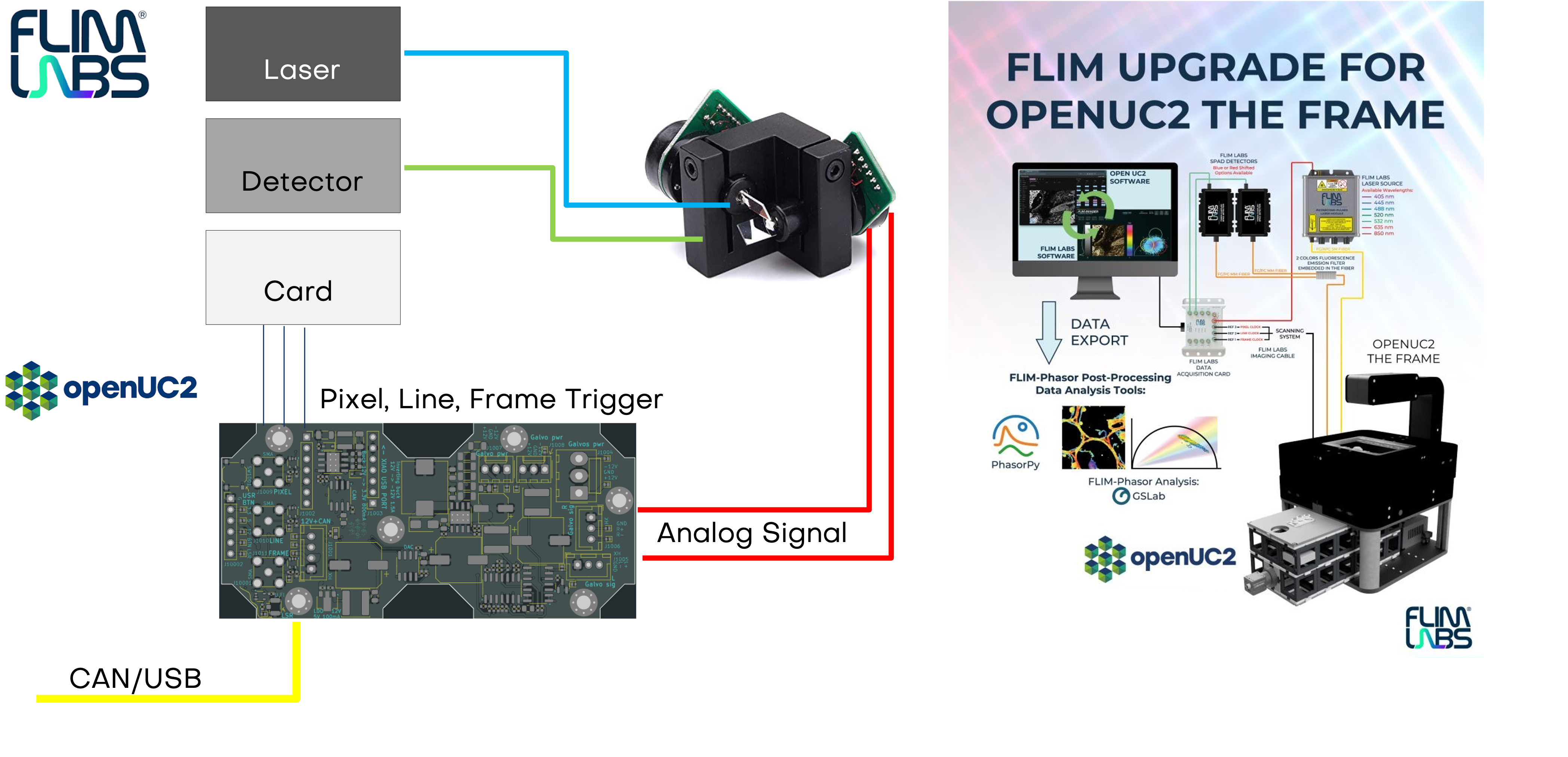
System blocks

The diagramm shows the current implementation of the triggering in combination with the FLIMLabs card. The openUC2 Galvo Scanner driver board relies on communication from the openUC2 CAN bus.

Optics (high level)

We define our simple laser scanning system bsaed on three principles that we tried to embedd into our optical setup:

1. A collimated excitation beam (single-mode fiber collimated that is imaged into the BFP of the exciation objective).
2. The galvo pivot (in our case we have two galvos, so it's the center between the two moving planes) is imaged into the objective back focal plane (BFP) so that a change in angle is translated in a shift of the focus in the sample plane.
3. The fluorescence focus is coupled efficiently into a detection fiber feeding the FLIM electronics.

This results into:

• Excitation: laser(s) -> single-mode fiber -> fiber collimator -> beam combiner (optional) -> galvo X/Y
• Scan relay: scan lens (short f - we actually don't use a scan lens yet, maybe soon. This would produce a linear deflection of the beam based on the mirror angle) + relay lens (longer f) as a telescope -> objective BFP
• Microscope head: dichroic for epi excitation and emission separation, objective, sample
• Detection: emission filter(s) -> coupling lens -> multimode fiber -> FlimLabs card input
• Filters: a proper set of excitation, emission and dichroics for the exictaiton/emission fiber

How this looks like:

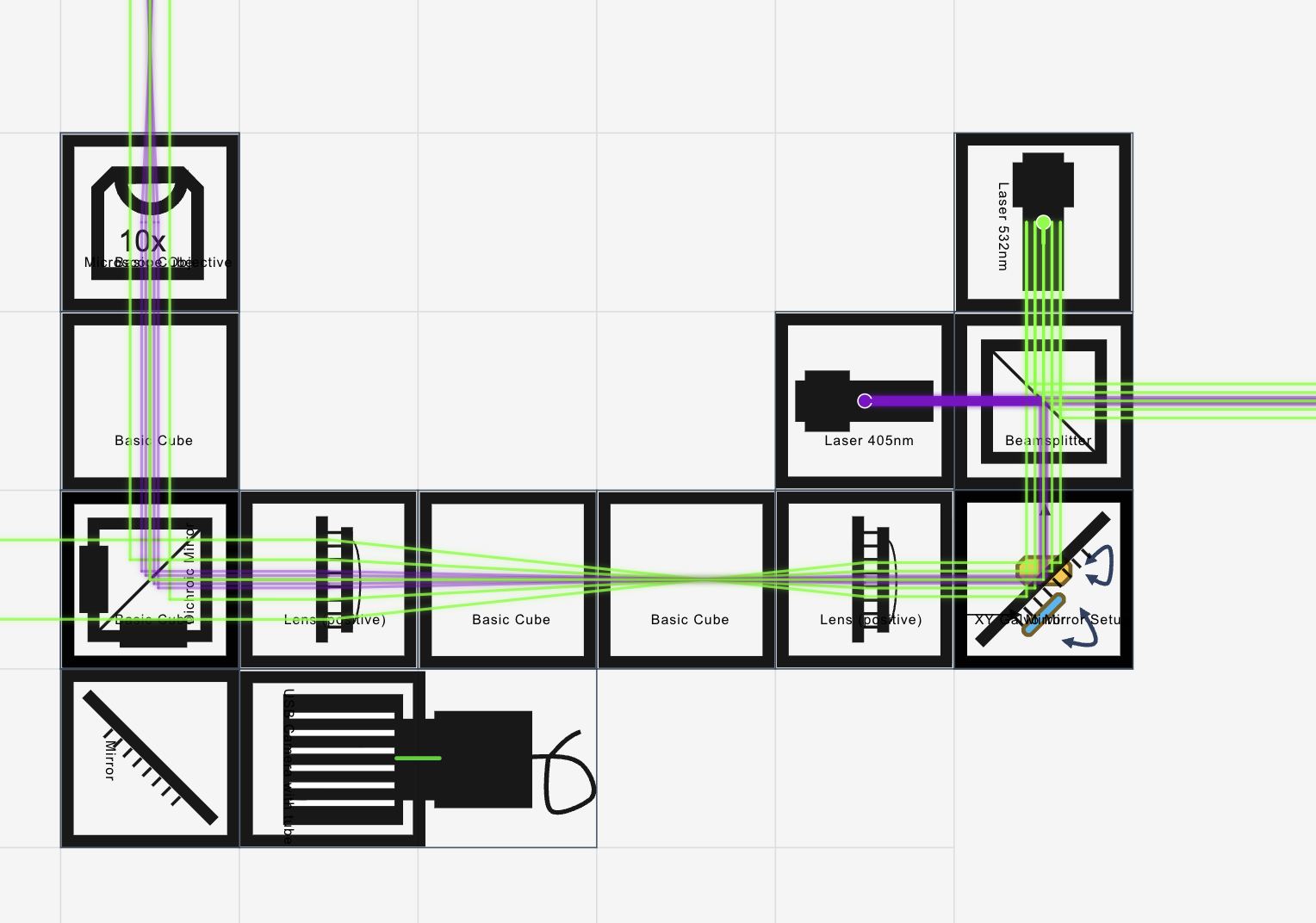
This is also available through our openUC2 Configurator.

Core optical principle (why “galvo in the BFP”)

If the galvo is conjugate to the objective pupil, the beam rotates around the pupil center. That produces a lateral shift of the focal spot in the sample plane without the beam walking across the pupil, and it keeps spot quality more constant across the field.

A useful small-angle relationship:

• A mirror deflection changes beam angle by about 2 theta
• The scan relay telescope scales angles
• The objective converts angle at the pupil into position in the sample plane

A compact approximation is:

$$[ x_{sample} \approx f_{obj}\cdot\theta_{obj} ]$$

and with a relay telescope of magnification (m=f_2/f_1):

$$[ \theta_{obj} \approx \frac{2\theta_{galvo}}{m} ]$$

So:

$$[ x_{sample} \approx f_{obj}\cdot \frac{2\theta_{galvo}}{m} ]$$

This is why changing relay focal lengths changes your field of view at the same galvo drive. For the integration of the system into the FRAME, we have to adjust the "scan" and "tube" lens such that we arrive in the BFP of the objective which is quiet "high" up in the FRAME.

This is how it looks like in the FRAME:

Build order that saves time

Do not start with scanning. First make the static beam perfect.

Step 1: Prepare the excitation beam (scanner off)

• Launch from the single-mode fiber collimator and make the beam collimated.
• Check collimation by measuring beam diameter near and far (for example 10 cm vs 1 to 2 m or use a an Ed shearing plate). It should not change much.
• The beam is reflected by the kinematic dichroic/combiner cube
• Route the beam through the cube centers using your alignment tool and temporary targets.

If you use two lasers (405 and 532), combine them coaxially now:

• Align laser A through the system first.
• Insert the kinematic combiner and steer laser B onto laser A.
• Verify coaxiality at two distances (near and far) so the beams do not just cross.

Step 2: Put the beam on the galvo correctly (scanner still off)

• Hit the center of the first mirror, then the second, with minimal clipping.
• Keep the mirrors as close as your module allows (reduces scan non-idealities compared to widely separated mirrors).
• Eventually move the galvo (by hand) to the position so that the beam walks towards the scan lens

Step 3: Build the scan relay (still off)

You need a scan lens plus a relay lens as a telescope that images the galvo pivot to the objective BFP.

Practical placement guide:

• Start with lens spacing close to ($f_{scan} + f_{relay}$) for an afocal telescope.
• Keep the optical axis straight and centered through the cubes.
• Add the dichroic and objective after the relay.

A good check before scanning:

• Put a temporary pupil viewer or a piece of paper near the pupil region if accessible. (e.g. camera)
• Even without motion, the beam should be centered and not clipped by apertures, dichroic clear aperture, or cube edges.

Step 4: Verify a tight focus at the sample

• Put a fluorescent slide or a scattering target at the sample plane.
• Focus until the spot is smallest and brightest.
• Only after that, enable a tiny scan amplitude and confirm the spot stays tight across a small region.

If the spot stretches with scan angle, treat it as a conjugation error (galvo not properly relayed to the BFP) or clipping.

Verification tip: The pupil plane is the one where the beam is not shifting laterally when you change the galvo angle. You can use a temporary camera or screen to find this plane. Ideally, this is an image of the scanner, so you can can insert a small target (e.g. a needle/hair) at the galvo pivot and see it in the pupil plane sharply focused.

Detection fiber and FLIM card coupling

Once the excitation spot and scanning geometry are correct, maximize detection efficiency. This step matters as much as the scan alignment for practical FLIM.

Procedure:

• Insert emission filters appropriate for your fluorophore(s) and lasers.

• Place the coupling lens that focuses emission into the multimode fiber.

• Use a stable fluorescent sample and keep excitation power constant.

• Iterate in small loops:

  • adjust the fiber coupler XYZ
  • adjust coupling lens position
  • very small tweaks of the kinematic combiner only if needed (avoid breaking coaxial excitation)

A helpful workflow is to scan a small ROI and maximize the mean count rate rather than chasing a single-point reading. It averages out speckle and small sample inhomogeneity.

Hint: It can be useful to use a second fiber-coupled laser in tandem for alignment. A bright red laser (e.g. 635nm) is easy to see and align through the system, then switch to fluorescence for final optimization.

Timing and electronics integration (scanner to FLIM)

Your scan electronics need to do two jobs: generate smooth analog scan signals and provide reliable digital timing for pixel binning.

A typical command for the GalvoScanner:

{"task": "/galvo_act", "config": {"nx": 256, "ny": 256, "x_min": 500, "x_max": 3500, "y_min": 500, "y_max": 3500, "sample_period_us": 1, "frame_count": 10, "bidirectional": 1}}

The section about the firmware in the UC2-ESP32 repository can be found here.

Key requirements for FLIM mapping:

• The FLIM card needs a consistent way to assign detected photons to pixels.
• If you do bidirectional scanning, you must handle line direction reversal in software or timing.
• Flyback photons must be excluded, either by blanking the laser or by gating them out in binning.

Keep the timing generated by the scan controller as the single source of truth. It reduces drift between scan position and photon assignment.

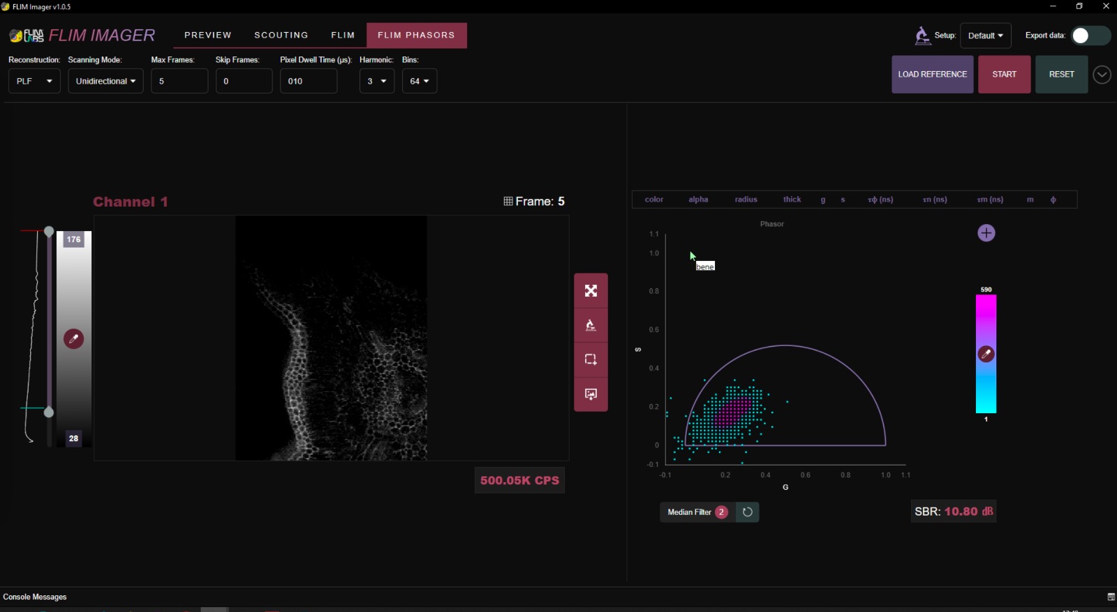
Software workflow in ImSwitch

Expose the parameters that directly change sampling and lifetime quality:

• scan mode: unidirectional or bidirectional
• frame size: Nx, Ny
• dwell time per pixel
• scan amplitude X and Y (field of view)
• flyback fraction or flyback timing
• binning (spatial, temporal) and minimum photons per pixel
• lifetime method: fit model or phasor (depending on what you use downstream)

A clean acquisition sequence is:

1. arm FLIM acquisition
2. start scanner waveforms and timing outputs
3. record photon events while timing defines pixel bins
4. compute intensity and lifetime maps

Validation experiments

1. Uniform fluorescent slide Expect nearly uniform intensity and a lifetime map that is spatially consistent within noise.

2. Sharp edge or sparse beads Expect higher contrast and reduced background compared to widefield. This is where fiber pinhole behavior becomes obvious.

3. Two dyes with different lifetimes Even if intensity looks similar, lifetime contrast should separate regions.

Result

This is a result acquired with the current FLIM version at 488nm excitation on an 10x, NA 0.3 objective.