CourseBOX: Light Microscopy and Optical Alignment (Infinity Optics)
This is the alignment procedure of the experiments with infinity-corrected optics. If you are looking for the finite-corrected setups click here, but this page is more complex and up-to-date.
It is more than just an alignment guide - we will also tell you about the observed effects! The explanations are marked with a ⭐
Find out how to build the CourseBOX in the BUILD_ME folder and try the experiments yourself.
Here you find the guidelines to show these experiments:

⭐ Why to switch from finite optics to infinity optics? Infinity imaging systems are much more flexible and practical than finite-corrected systems. Probably the biggest advantage of an infinity system is that you can add filters, beamsplitters and other components (but not lenses!) in the optical path without shifting the position of the image.
First experiment: Compound Microscope and Illumination of the Sample
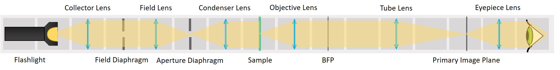
This experiment demonstrates the essential parts of a transmission light microscope and explains the concept of conjugate planes. We will start with a simple direct illumination and build up to a proper Köhler illumination, while observing the advantages and disadvantages of each illumination type.

Second experiment: Abbe Diffraction Experiment
Click here to watch a video of the UC2 Abbe Experiment on our YouTube channel!
The famous Abbe Diffraction Experiments shows how diffraction of light by a specimen (and interference with the illuminating light) creates an image and how collection of diffracted light defines the resolution of the microscope. With this setup it is possible to view both sets of conjugate planes at the same time, on a camera or a screen.
We provide different apertures that can be placed in the BFP. We use a very fine fish net as a sample here. You could try a net like this one. Another idea is to try one of these plastic tea bags. Or of course you can take a proper diffraction grating (but where's the fun in that?). If you have other ideas for cool samples, let us know!
Skip to the Abbe Diffraction Experiment
 This tutorial will lead you step-by-step through the alignment of the Compound Microscope, different Illumination types and the Abbe Diffraction Experiment and explain the optical phenomena you observe with these systems
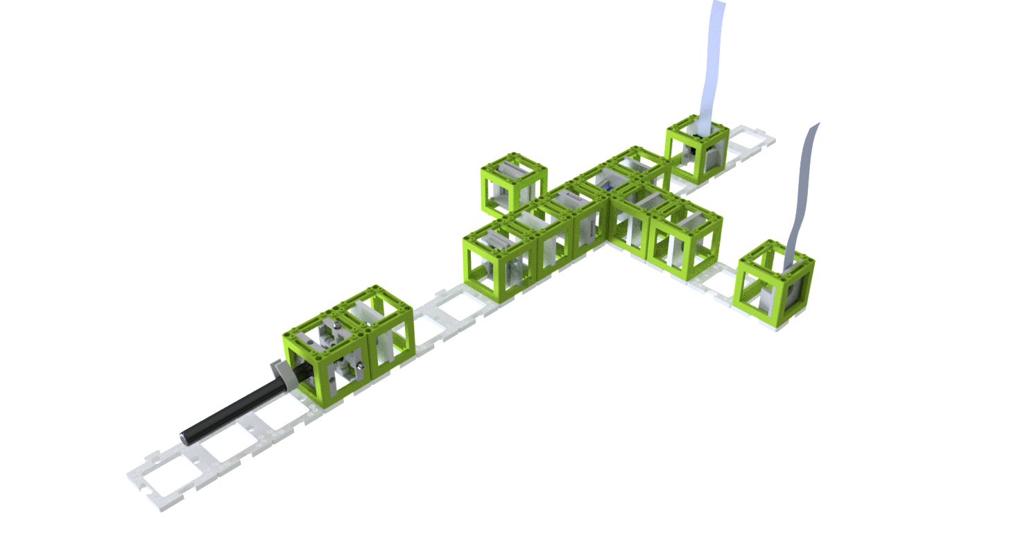
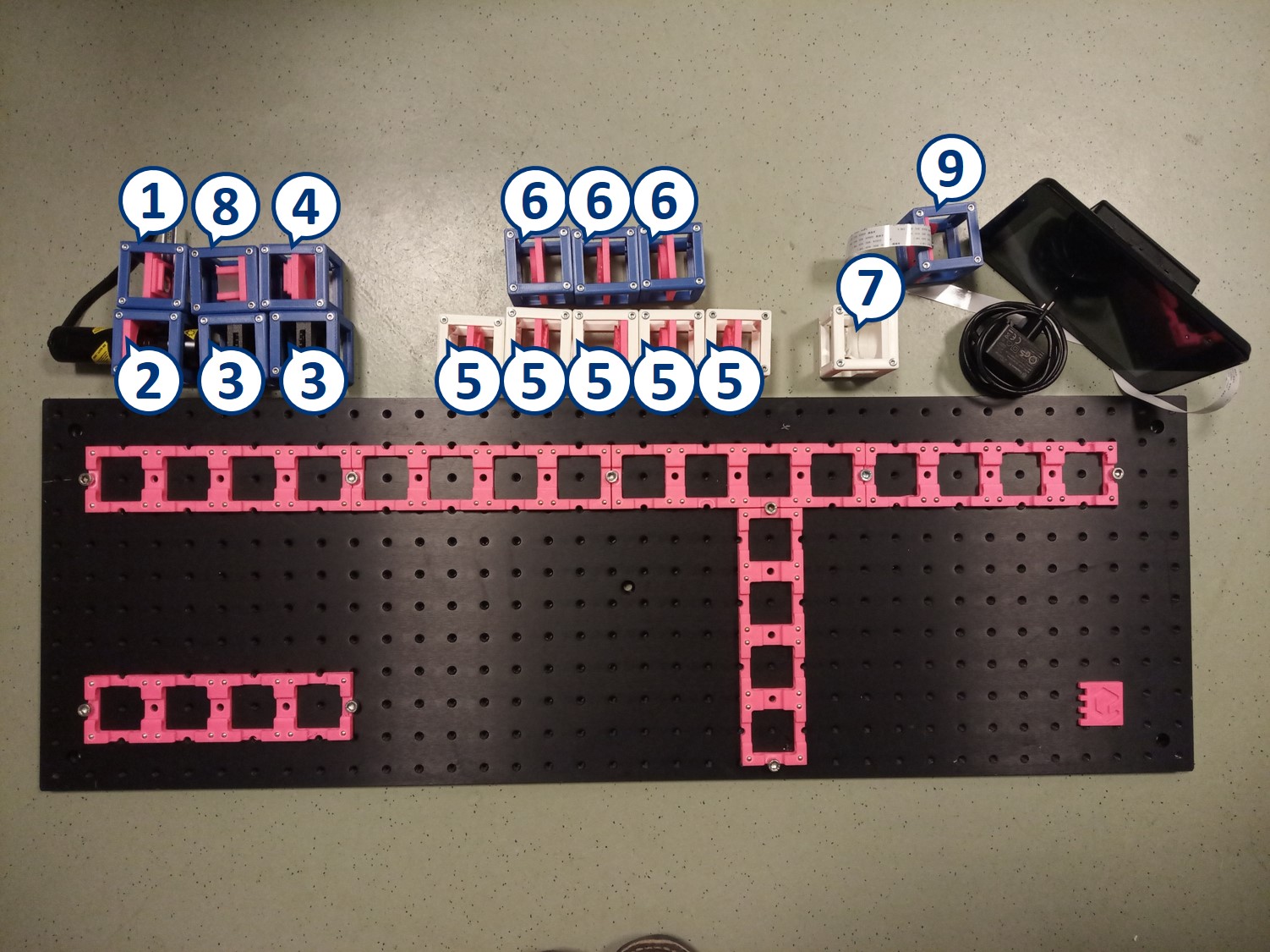
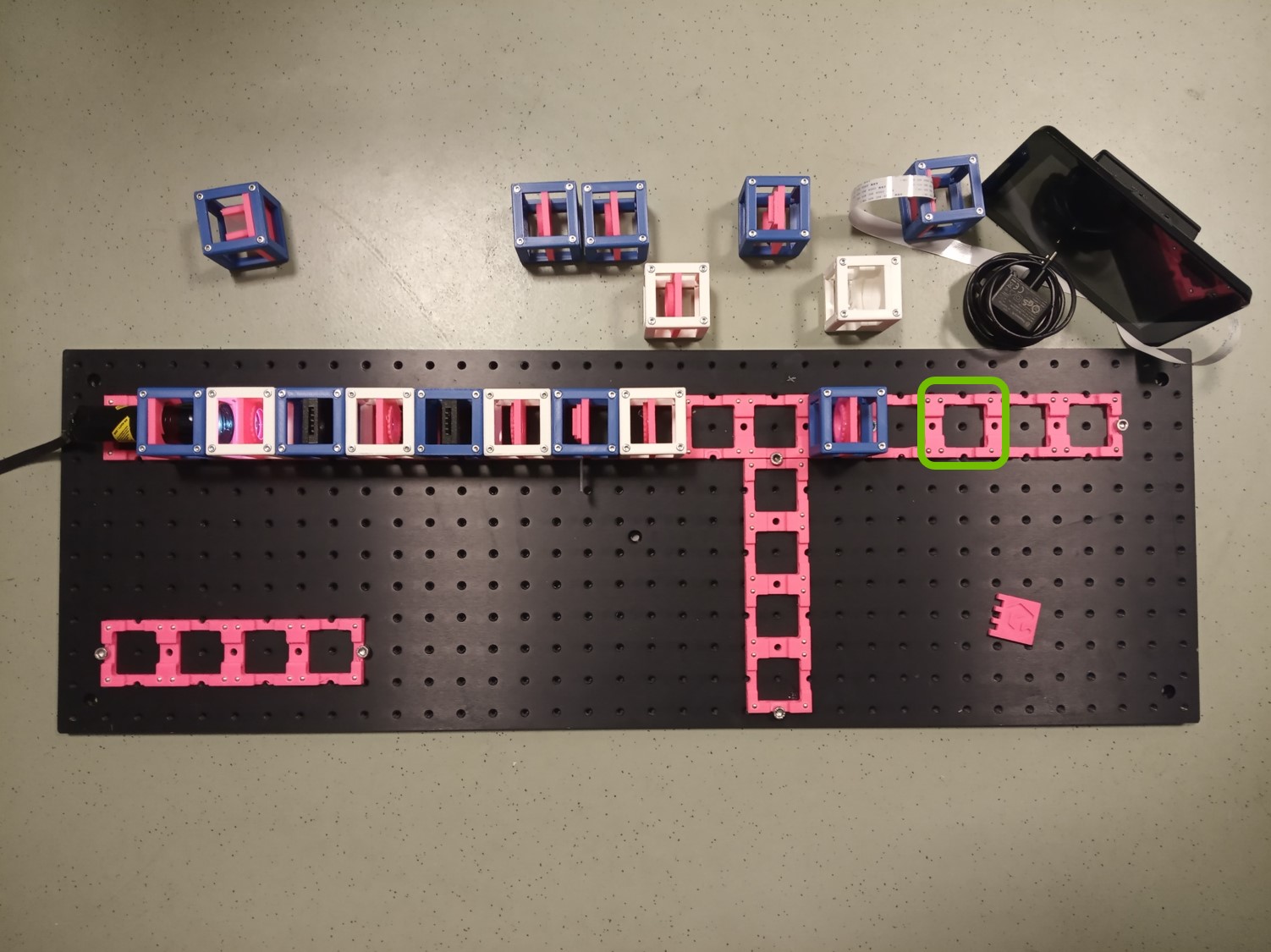
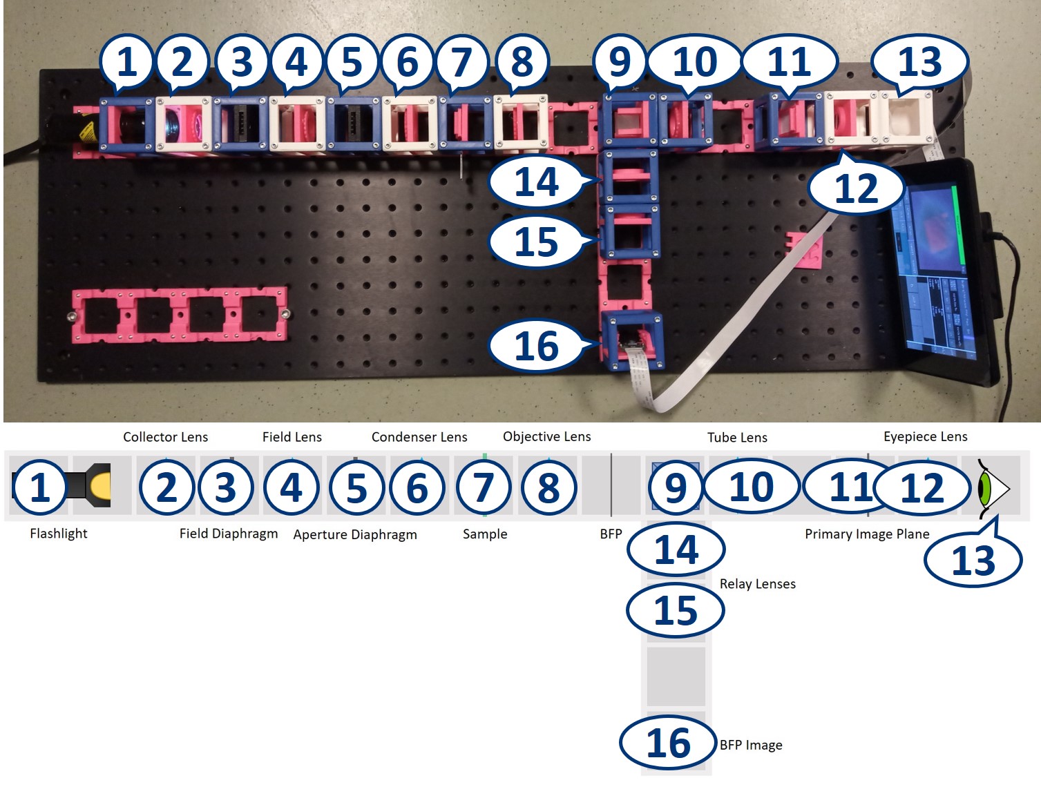
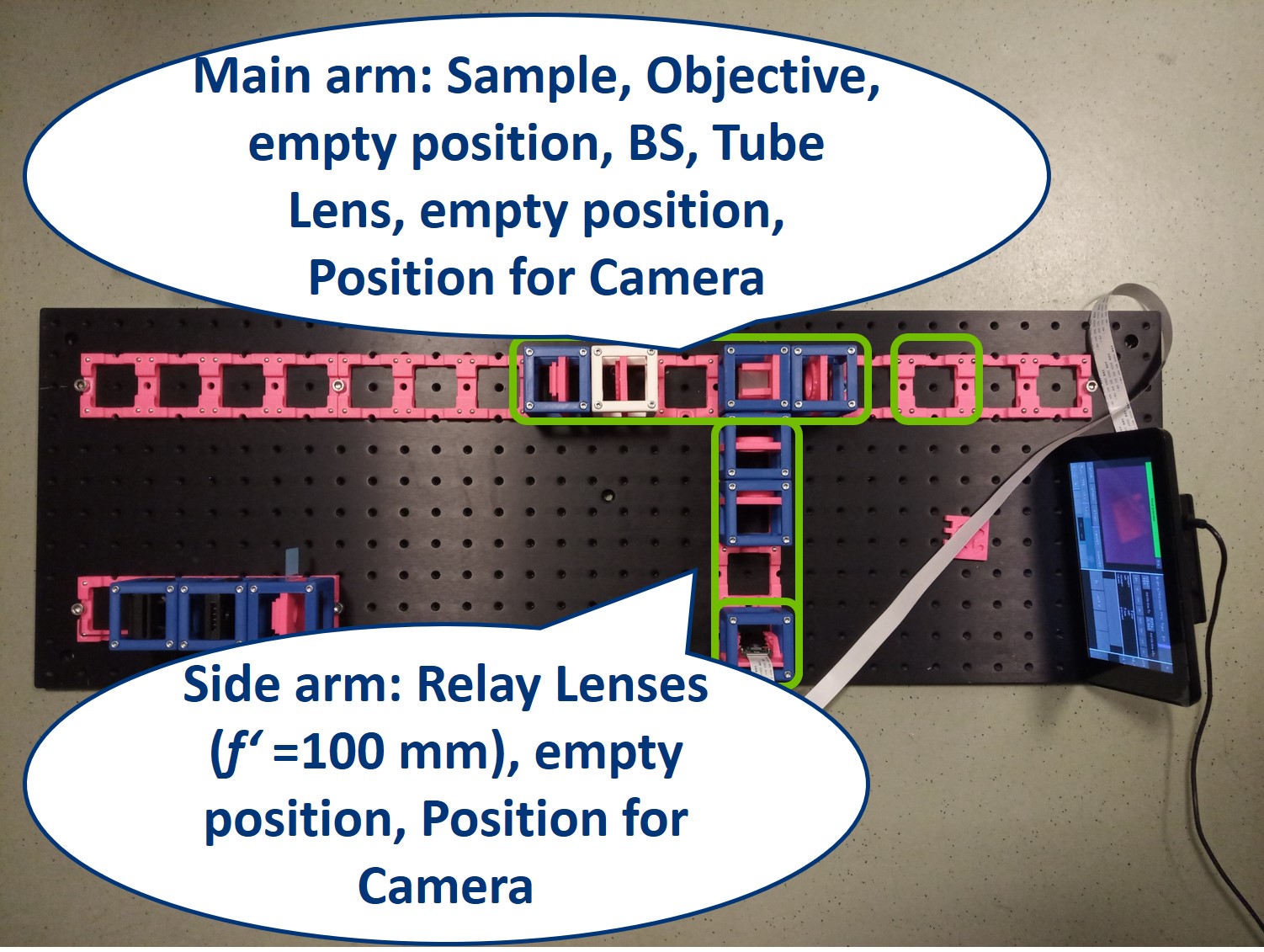
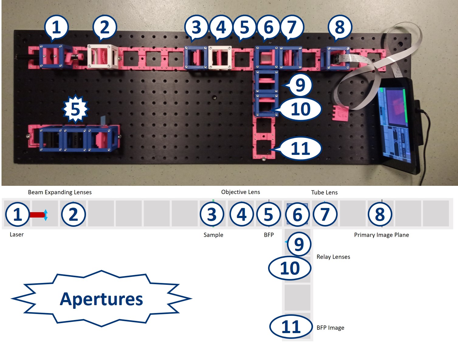
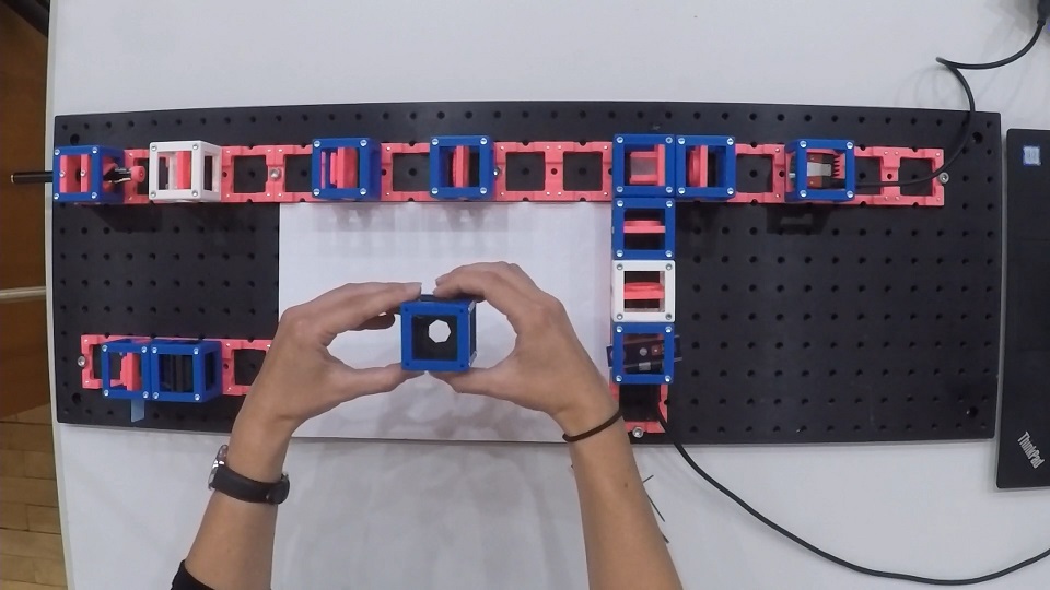
- Start with five 4×1 baseplates mounted as shown in the picture to an optical breadboard or to a wooden board. Prepare the following cubes:
- Sample Cube (1)
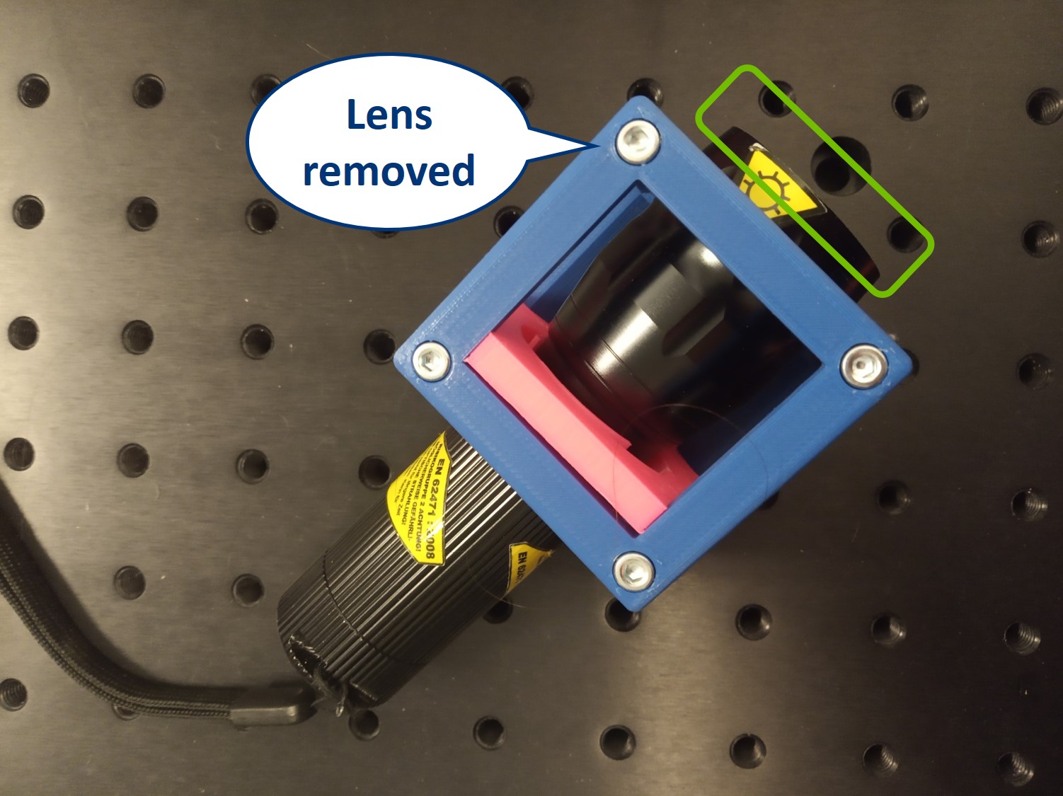
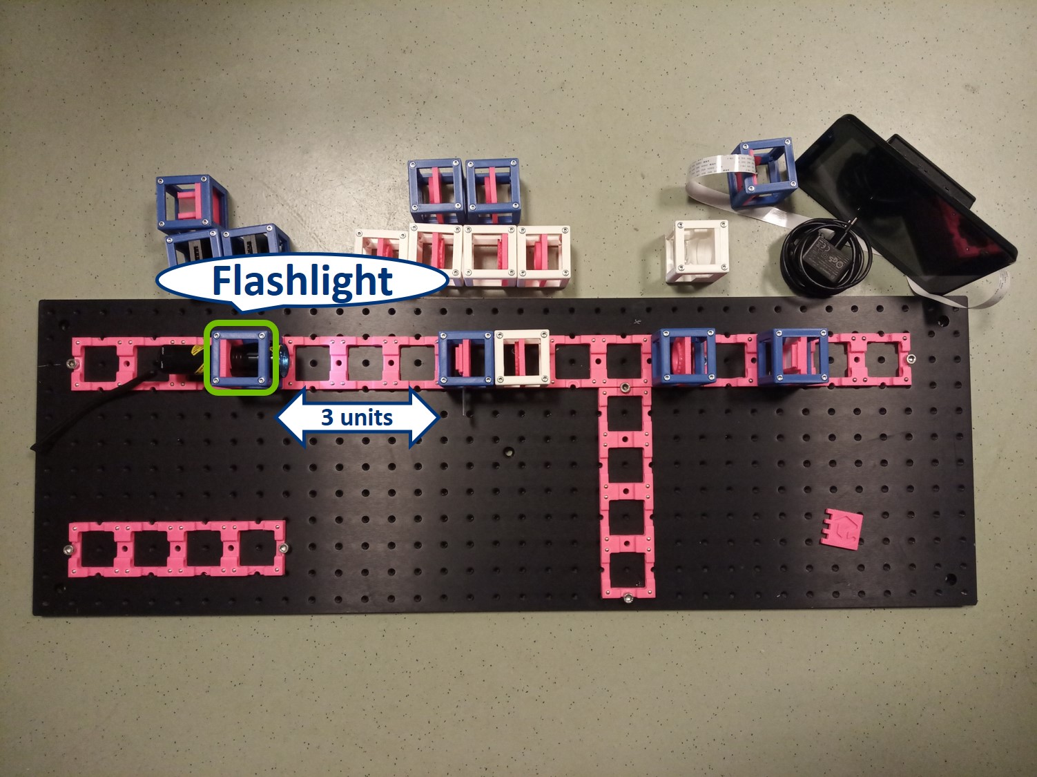
- Flashlight Cube (2) - Use the flashlight WITHOUT its lens in all the experiments
- 2× Circular Aperture Cube (3)
- Screen - Sample Holder Cube with white paper (4)
- 5× Lens Cube with 50 mm lens (5)
- 3× Lens Cube with 100 mm lens (6)
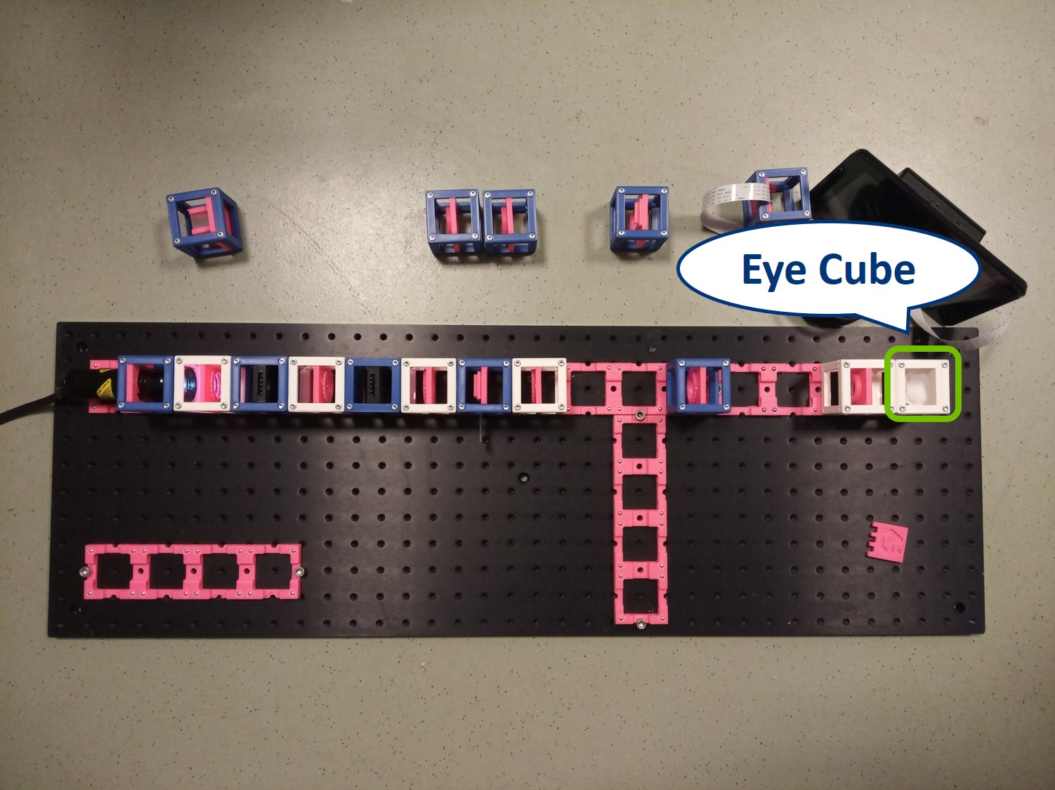
- Eye Cube (7)
- Beamsplitter Cube (8)
- Raspi Camera Cube (9)
Also prepare:
- Raspberry Pi
- UC2 Alignment Tool
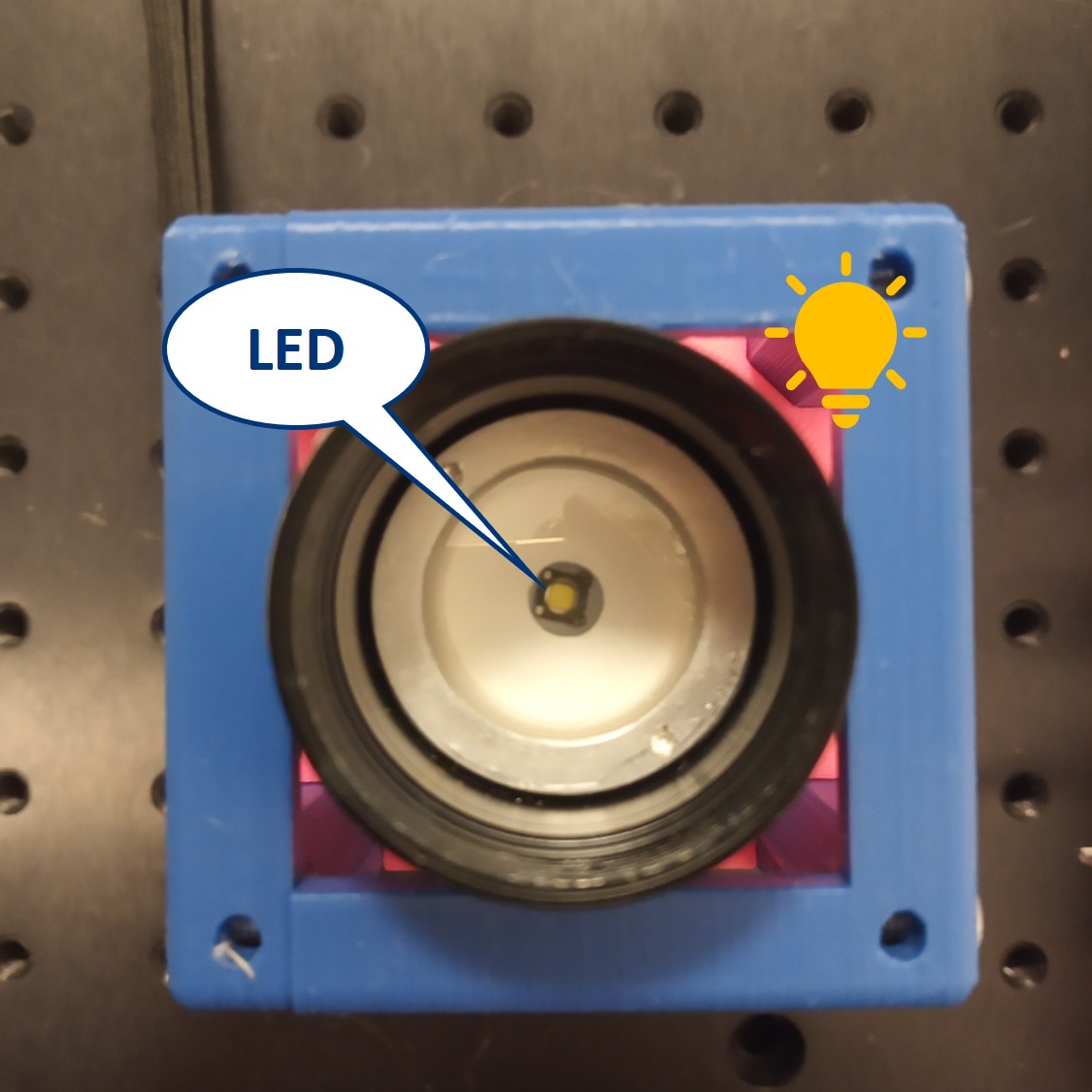
⭐ Why to use the flashlight without the lens? It would be one too many lenses in out system. In order to image the LED with our illumination optical path, we need to have access to the bare LED. Before you start building the microscope, remove the lens from the flashlight.
⭐ Infinite conjugate imaging system
We form a real image of the sample by a method known as infinite conjugate system. If the object is placed in the focal plane of a lens, its image is formed in the infinity, because the rays diffracted by the object are parallel after the lens. If a second lens is placed after the first one, it captures these parallel rays and a real image of the object is formed in the focal plane of the second lens. The magnification of an infinite conjugate system is given by
M = -f2/f1
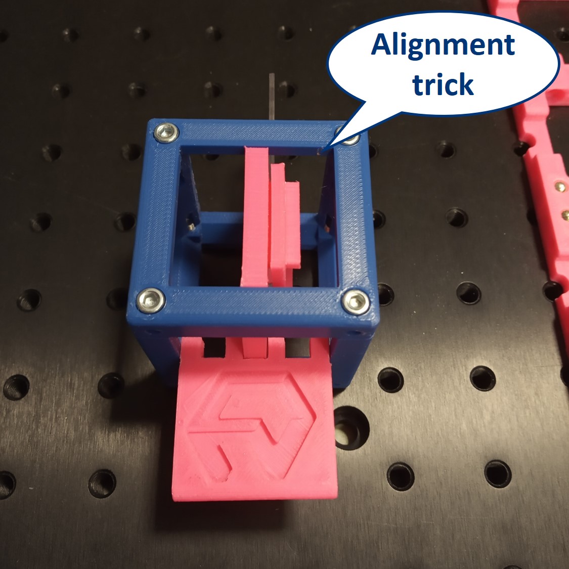
- Start by placing the sample - we will build the microscope around it.
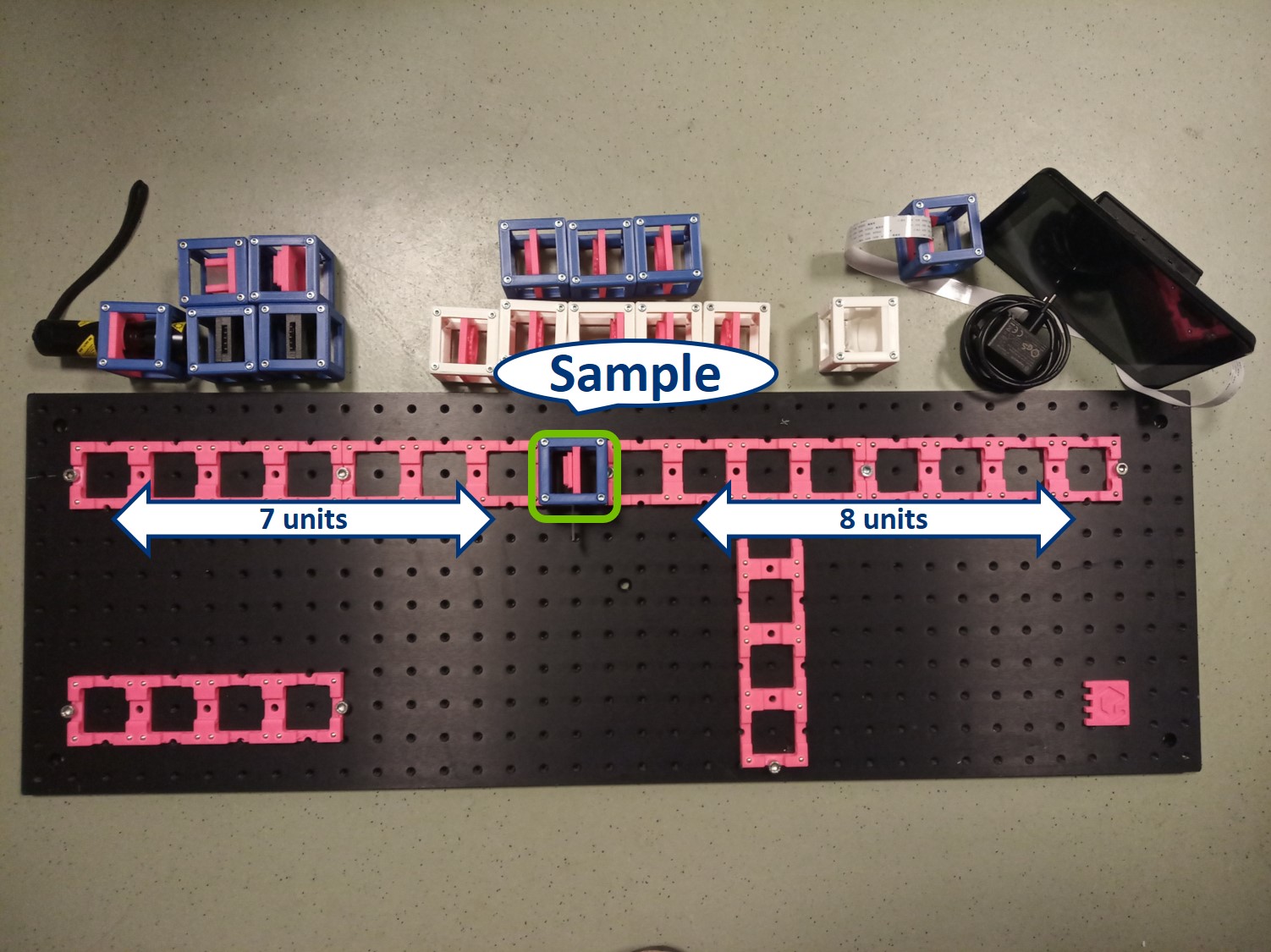
- Alignment trick: Use the Alignment Tool and align all inserts (Sample, screen, lenses) to the centers of the cubes as you place them on the baseplate. This ways, because we use 50 mm and 100 m lenses, you will have the whole setup roughly pre-aligned from the beginning.
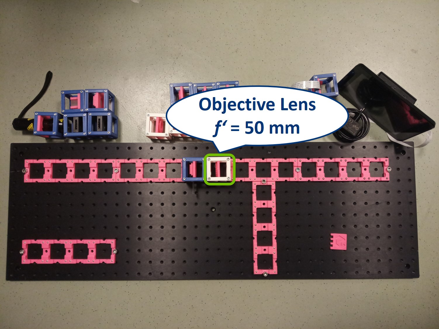
- Place the objective lens. It is a single plano-convex lens with f' = 50 mm.
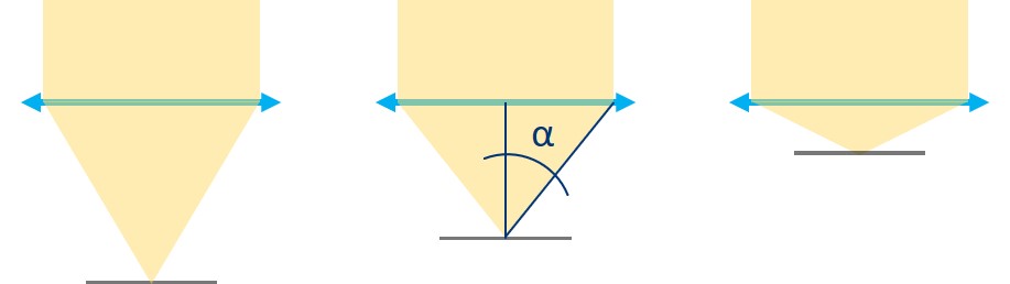
⭐ Numerical Aperture and Resolution
The Numerical Aperture (NA) describes how much light coming from an imaged object is captured and focussed by the objective and determines the resolution of the system (and not just that). It is given by
NA = n × sin(alpha) ,
where n is the refractive index of the medium between the sample and the objective (here, in air, n = 1) and alpha is the angle of the between the optical axis and the steepest rays that are still collected by the objective. The angle alpha can be calculated from the focal length f' of the objective lens and its diameter d, because
tan(alpha) = 1/2 d / f' .
From the NA we can calculate the resolution of our imaging system. Physically, the resolution s the smallest distance between two point is the sample that are still imaged as two point. If the points are any closer, the will appear as a single point in the Image Plane. For the microscope here, we calculate the resolution as
R = 0,61 lambda / NA ,
where lambda is the wavelength of the illumination. Because we use a white light source, we take lambda = 550 nm, since this is roughly in the middle of the visible spectrum.
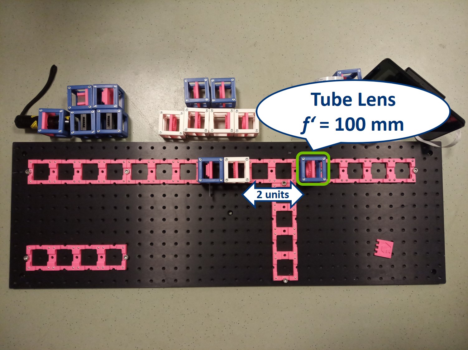
Place the tube lens. It is a single plano-convex lens with f' = 100 mm.
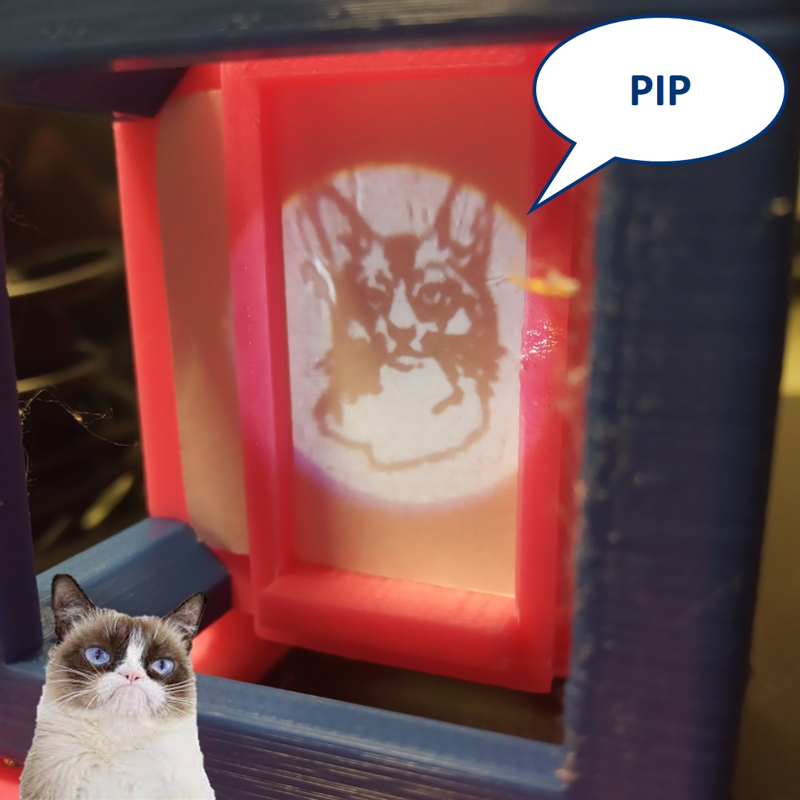
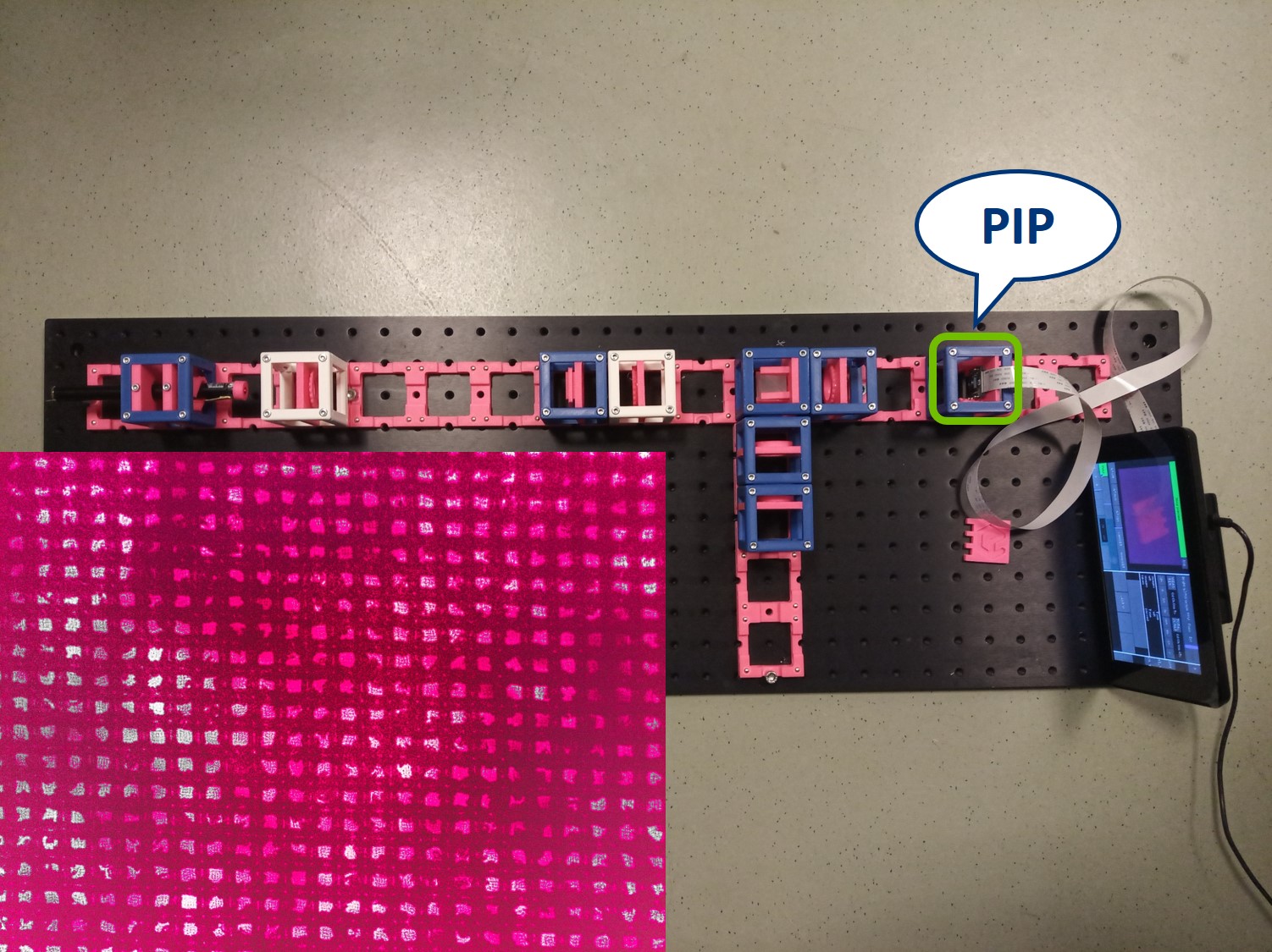
Place the Primary Image Plane (PIP) in the focal plane of the tube lens. Use the Sample cube with white paper as a screen.
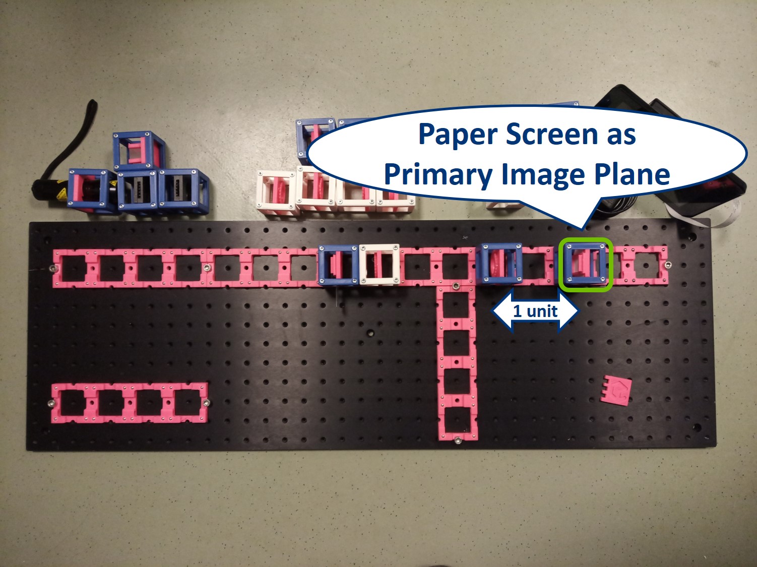
⭐ Now we have the imaging infinite conjugate system. The second lens can be placed at any distance from the first one, because the rays are parallel after the first lens. As long as the system is well aligned, the distance between the lenses doesn't really matter. Of course it shouldn't be across the whole room, because we would loose intensity and some of the marginal rays. Here we build it in such a way that the Back Focal Plane of the Objective coincides with the front focal plane of the tube lens, which is the most optimal way for Fourier imaging and it will be convenient for the next steps.
⭐ Numerical aperture of our imaging system equals to NA = 1 × sin(alpha) , with alpha coming from tan(alpha) = 0,5×25,4 / 50. Therefore our NA = 0,25. The resolution of our microscope is then R = 0,61×0,550 / 0,25 = 1,342 um .
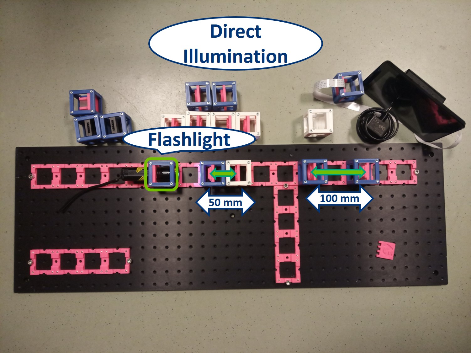
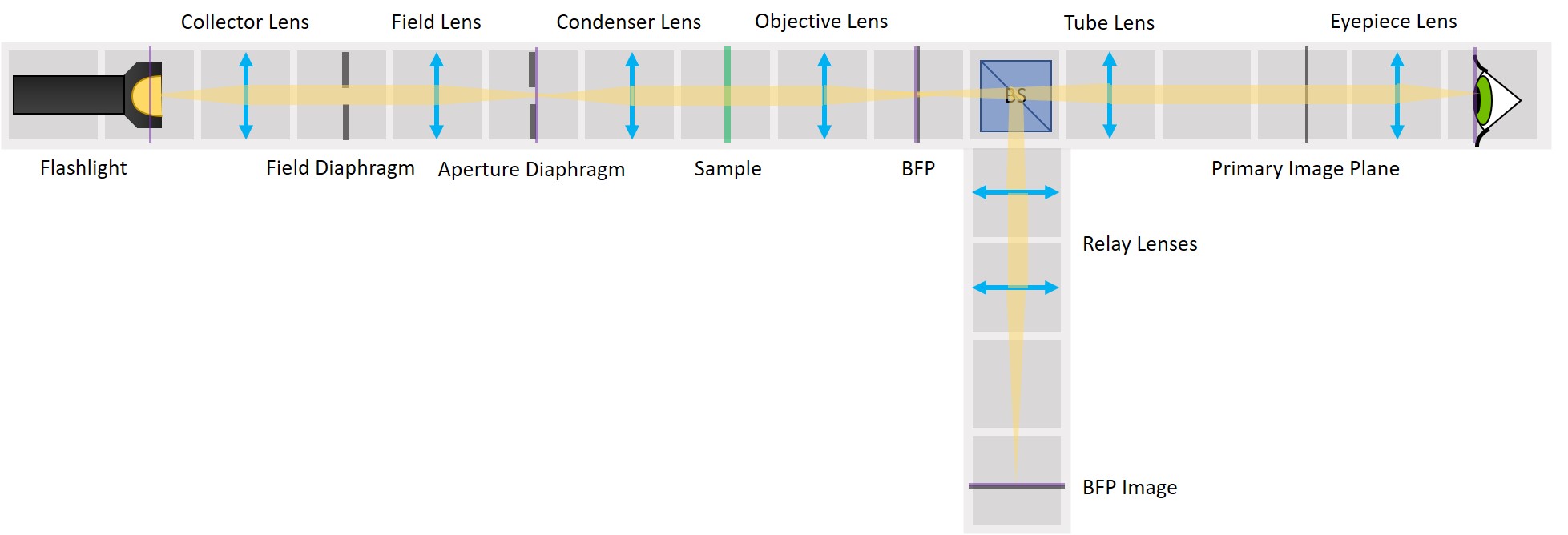
⭐ Direct Illumination
To start with the simplest way of illuminating a sample, we place the flashlight, our light source, close to the sample. This way we can see an image of our sample on the screen. This is called Direct illumination, but it's a very inefficient illumination type because only a small fraction of the light emitted from the source will actually hit the sample.

- Starting with Direct illumination: Use the flashlight WITHOUT its lens as a direct illumination source, its exact position is not that important. The Sample has to be in the front focal plane of the objective and the screen has to be in the back focal plane of the tube lens - you can use the I. Focussing Trick. Adjust the position of the inserts to focus the image on PIP - you can use the II. Focussing Trick.
- Focussing Trick I for infinity optics: How to make sure that a screen (sample, aperture) is in the focal plane of a lens? Place the Lens cube and the paper screen on a baseplate in roughly the aligned distance (depending on the focal length of the lens). Image something from the infinity on the screen with this lens. A good object in the infinity can be the clouds in the sky or a window on the other side of the room (at least 4-5 m away). Shift the Insert carrying your screen inside the cube to see a sharp image of the clouds/window/... Now you know the distance in which you want to have the component that is supposed to be adjacent to the lens.
- Focussing Trick II for general alignment: Firstly move the whole Sample cube with the screen in one direction (away from the tube lens). If the image sharpness in PIP improves, slide the insert in that direction. If the image sharpness in PIP gets worse, slide the insert in the opposite direction, towards the sample. Continue until you get a focussed image of your sample on the PIP.
- Alignment Check: When your imaging path is properly aligned, the distance between the objective and the tube lens doesn't matter, because the light rays between the lenses are parallel to the optical axis. Check this by moving the Tube lens and screen TOGETHER forwards or backwards by a baseplate-unit or two. The image on the screen must not change.
⭐ Now you can see that we were right about the infinite conjugate system.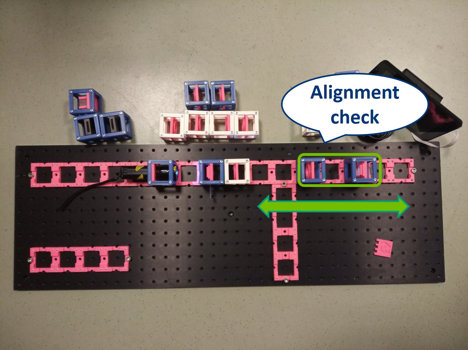
⭐ The magnification of an infinite conjugate system is given by M = - f2/f1 as we said. In infinity-corrected microscopes it is usually described as M = - fTube lens/fObjective for the imaging system. The magnification of our imaging system here is therefore M = - 100/50 = -2. We can see an inverted 2× magnified image of our Sample in the Primary Image Plane.
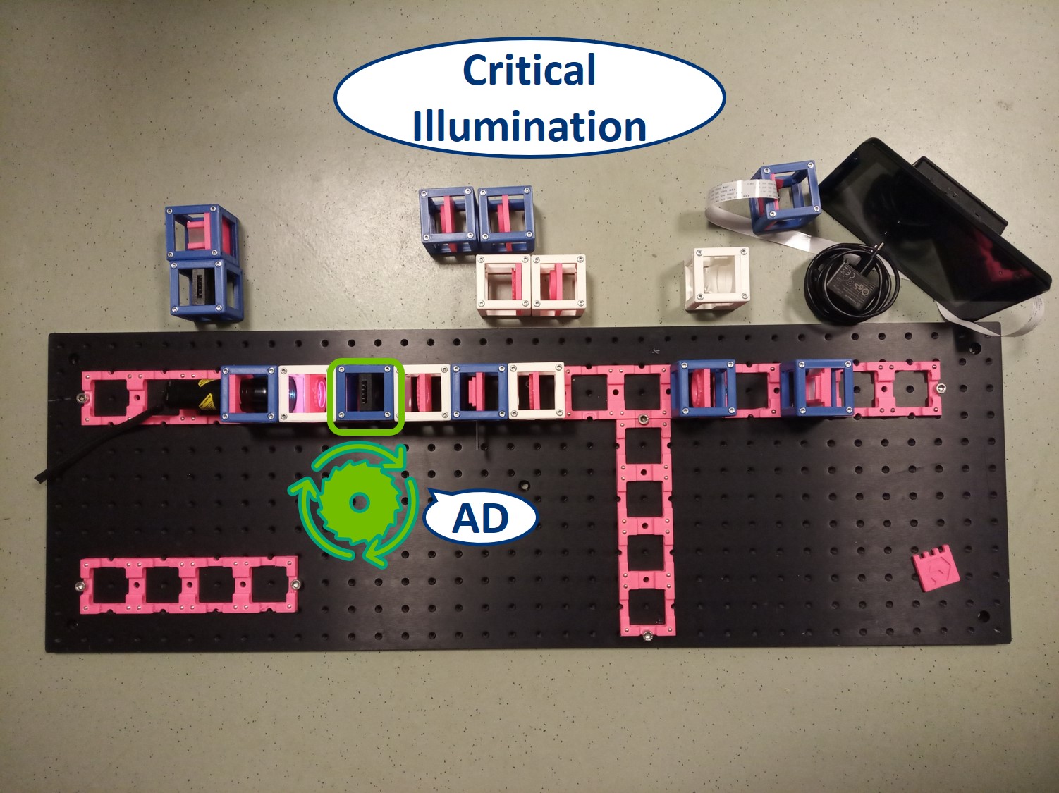
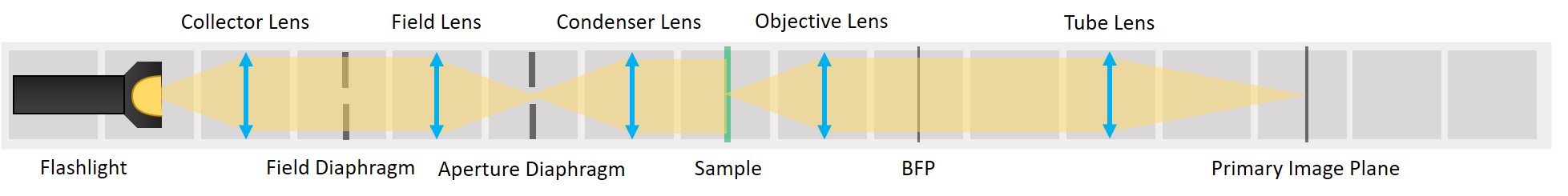
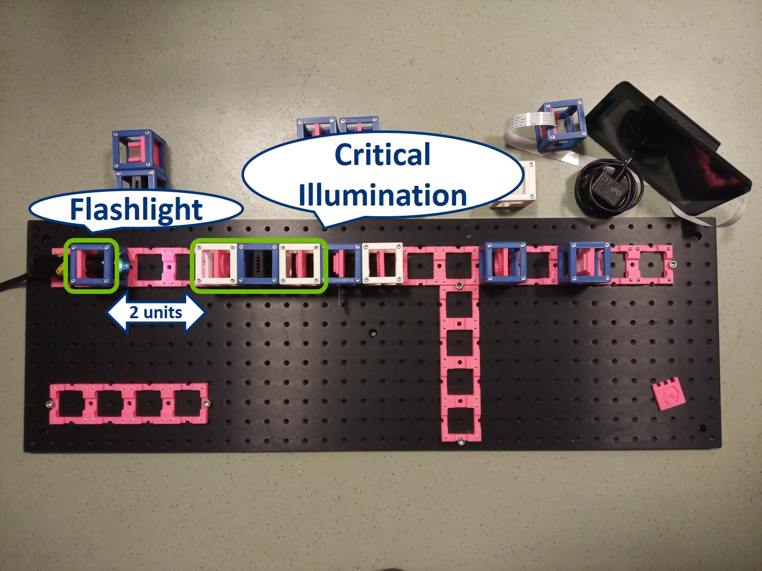
⭐ Critical Illumination
To capture all the light from the flashlight, we build a second infinite conjugate system on the illumination side of the sample. This will form an image of the flashlight's LED on the sample. This is called critical illumination. The advantage of having an infinite conjugate critical illumination is that we can include an Aperture diaphragm (AD). The AD limits the range of angles of the rays that illuminate the sample and therefore influences the resolution and contrast.

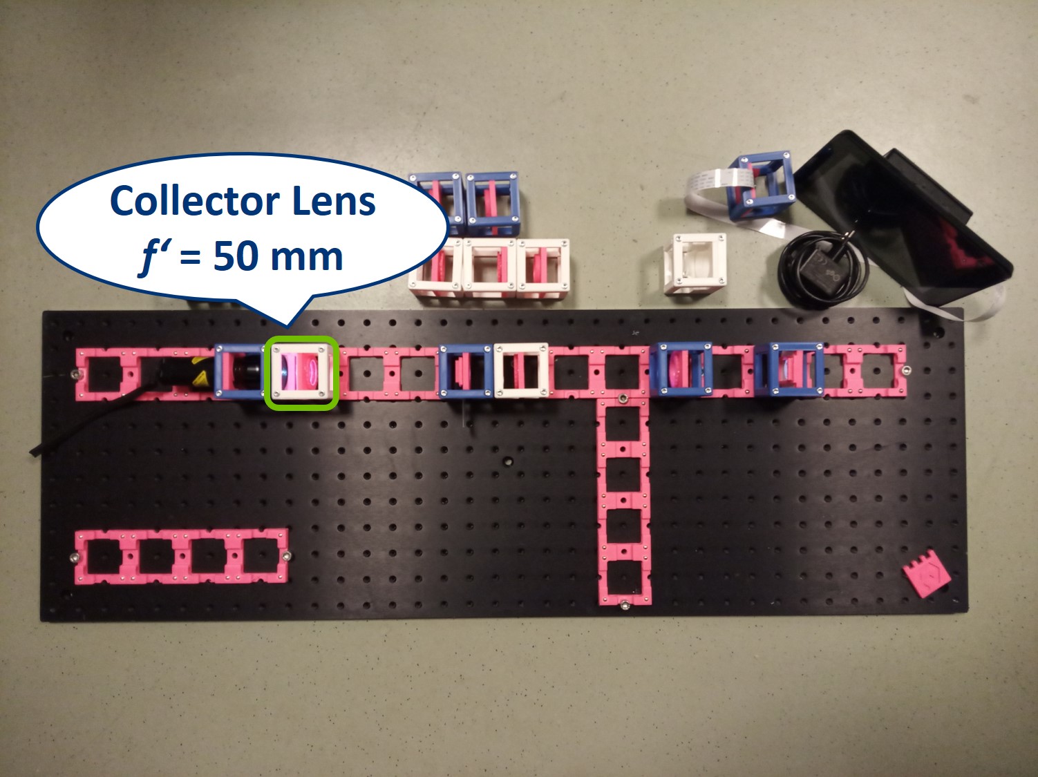
Building Critical illumination: Move the flashlight further from the Sample as shown in the picture.
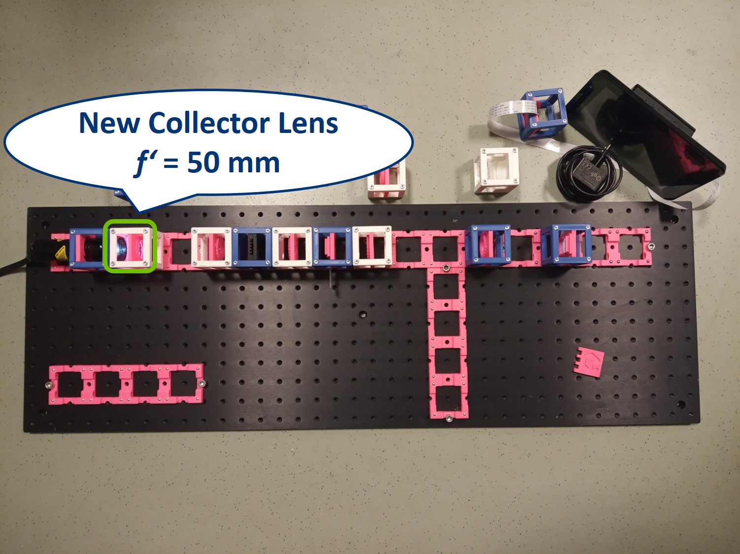
Place a collector lens next to the flashlight. It is a single plano-convex lens with f' = 50 mm.
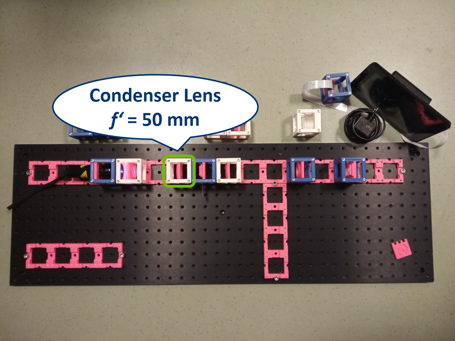
Place the condenser lens in front of the Sample. It is a single plano-convex lens with f' = 50 mm.
Place the Aperture Diaphragm (AD) between the collector and condenser. You can roughly align it to the center of the cube and precisely align it with the lenses using I. Focussing Trick. This is a microscope with critical illumination.
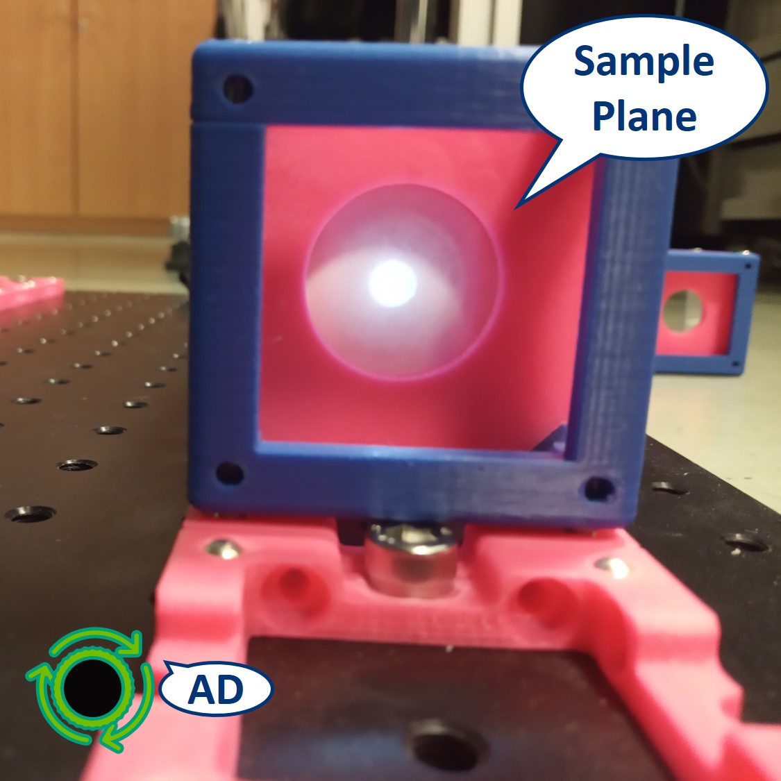
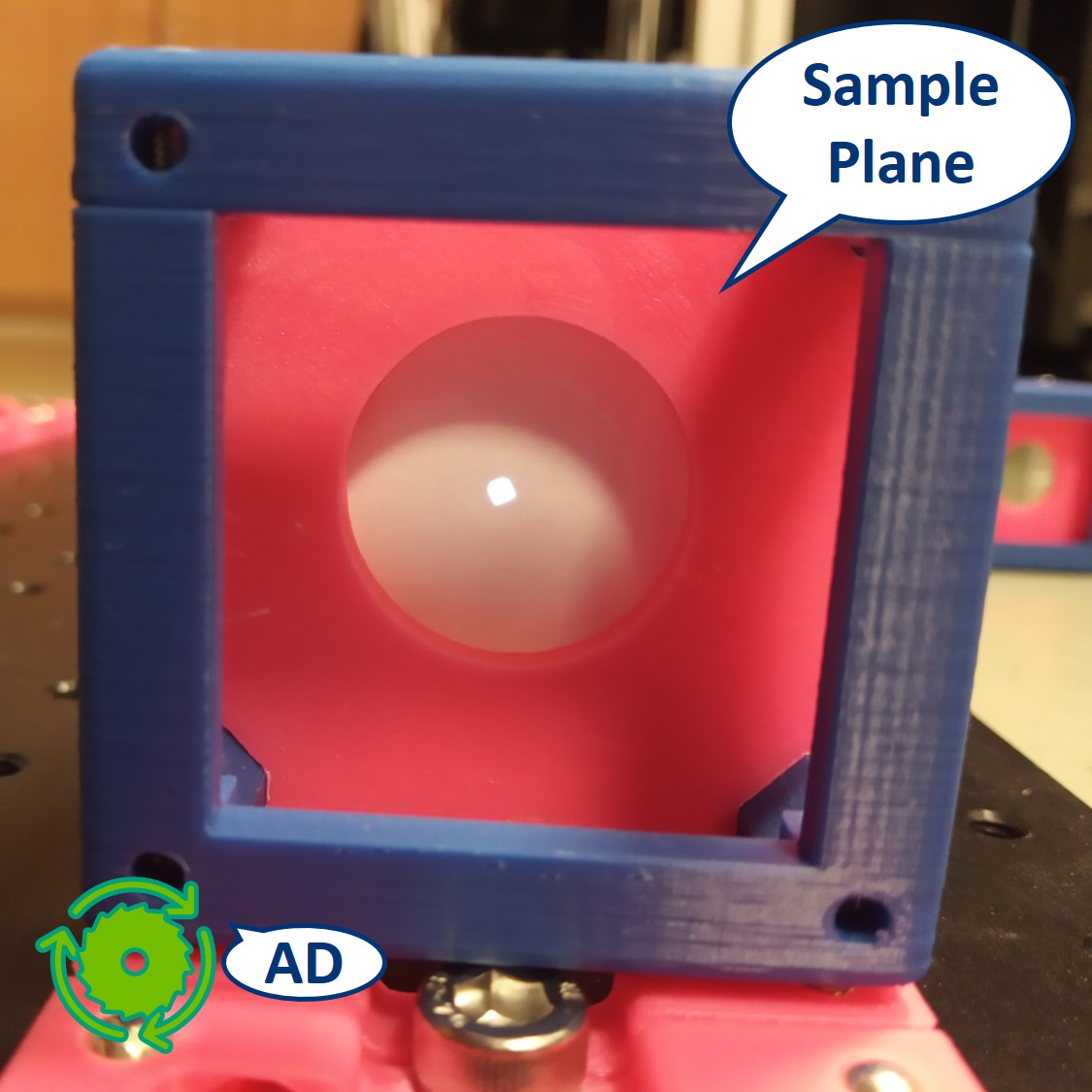
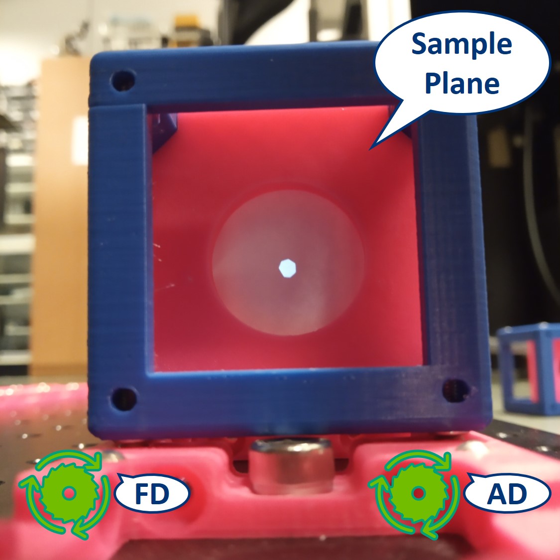
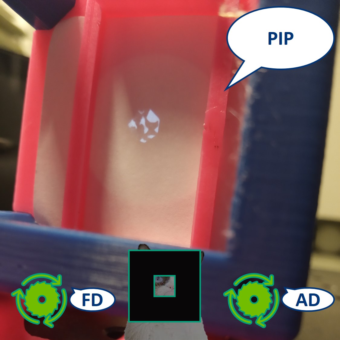
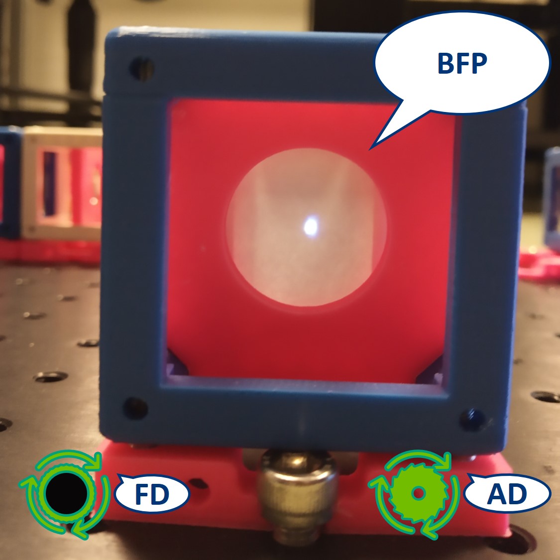
Let's have a look at the effect of the AD. You should be able to see it on the Sample itself but here we placed the paper screen in the position of the sample to be able to picture it.
The LED of the flashlight is now imaged directly on our sample. The flashlight used here is extremely bright and therefore the pictures shown here might look a bit misleading, because it wasn't possible to take a better, not oversaturated pictures.
⭐ Both the collector and condenser lens have focal length of 50 mm, therefore the magnification of this infinite conjugate system is equal to -1. We see an image of the LED, in real size but inverted, on the sample.
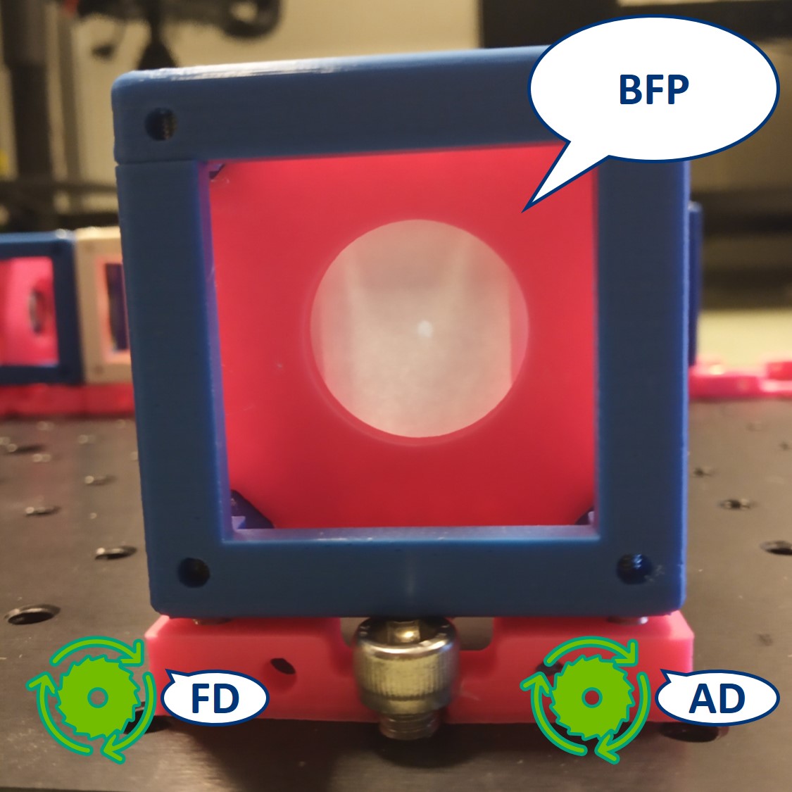
Top left: AD open, the spot is very bright.
Top right: AD closed, the spot seems smaller but it's just less bright. We can recognize the shape of the LED imaged in this plane.
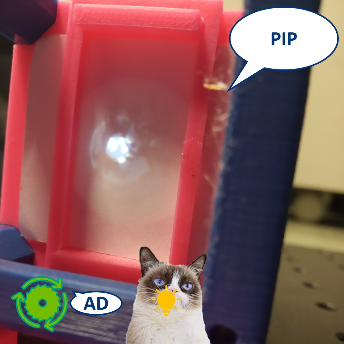
Bottom: In PIP, we seen the image of the LED over the image of the Sample.
⭐ The magnification of multiple infinite conjugate systems in a row is given by their multiplication. The image of the LED that we see in the PIP is given by MLED in PIP = MIllumination×MImaging = -1 × -2 = 2. We can see a non-inverted 2× magnified image of the LED in the Primary Image Plane.
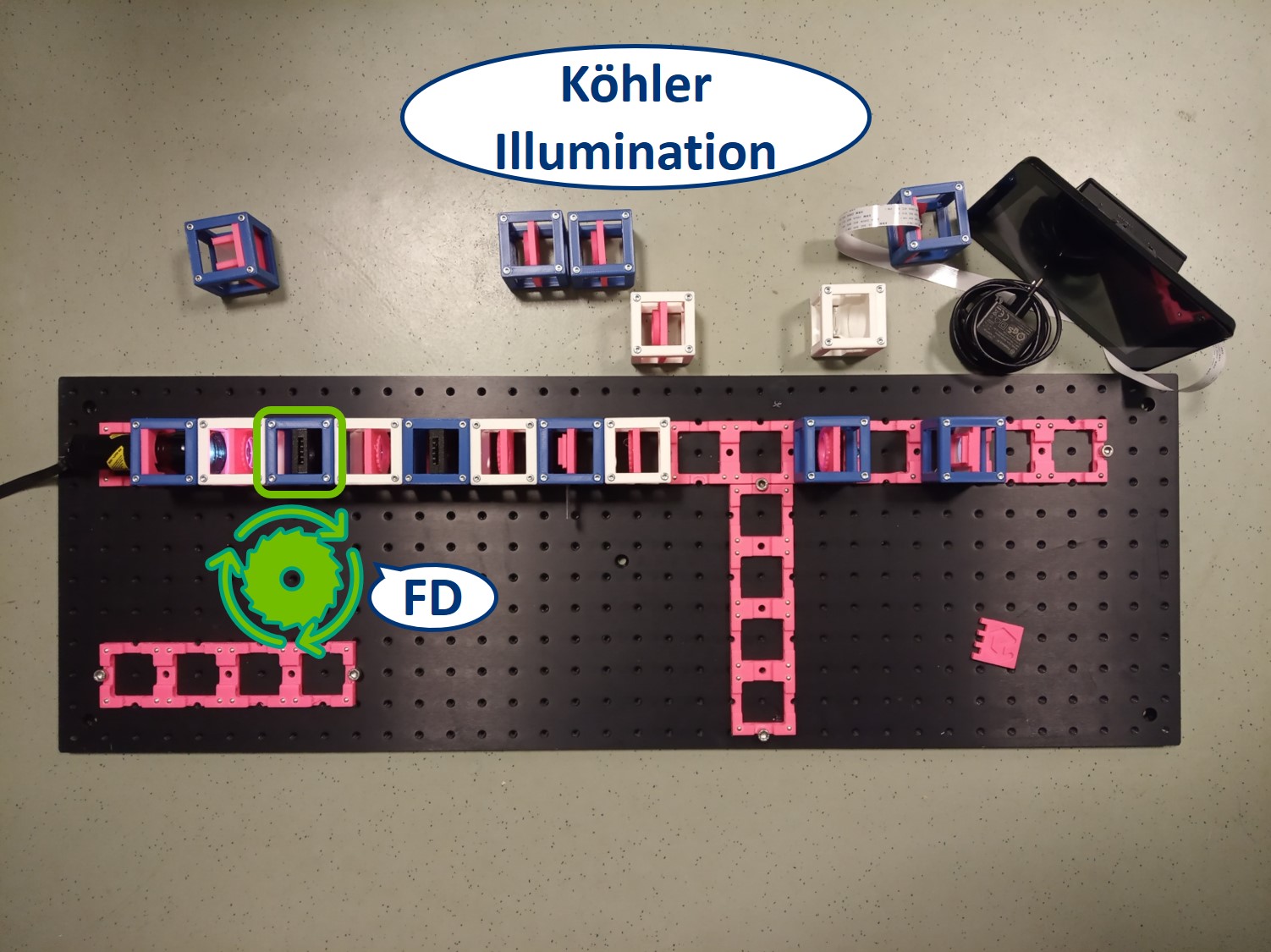
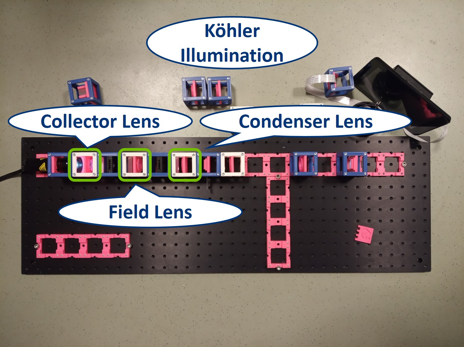
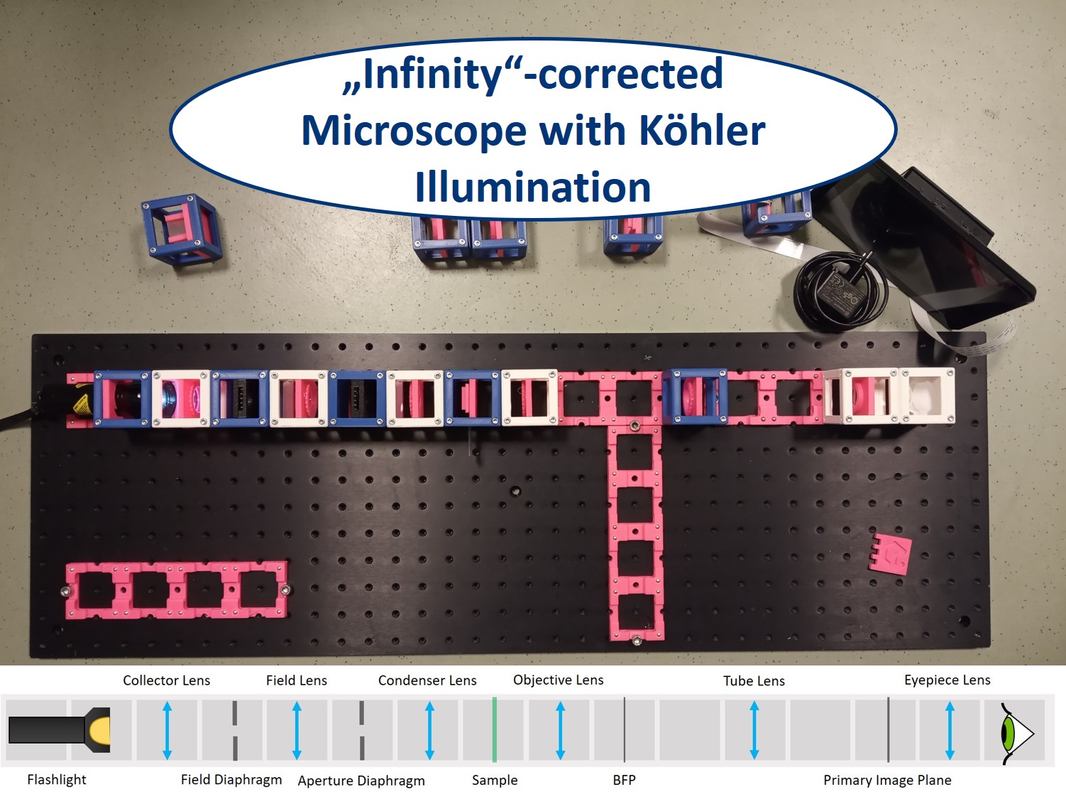
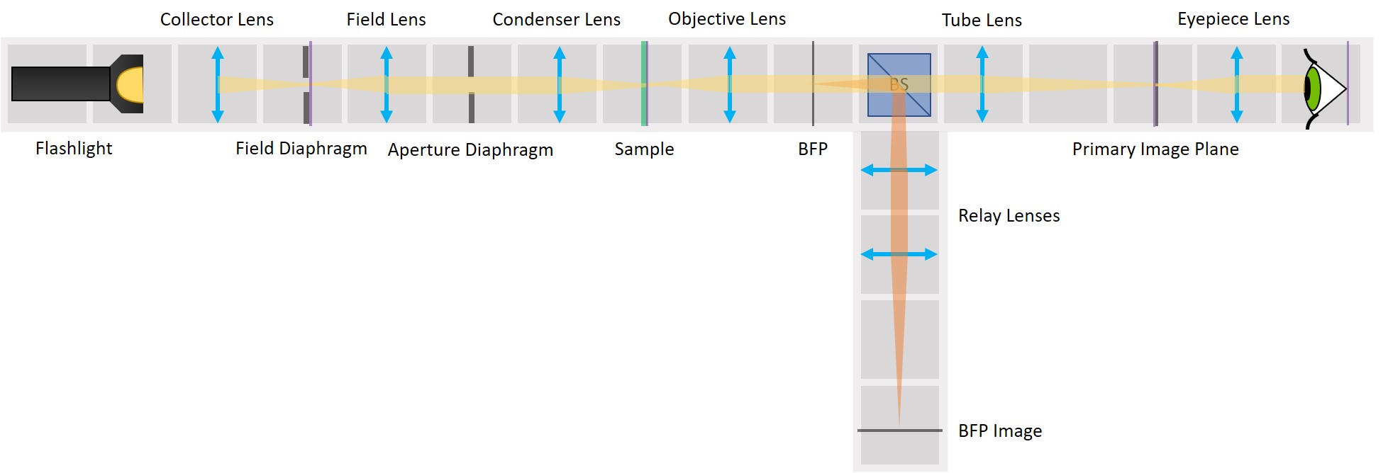
⭐ Köhler Illumination
With the critical illumination, the sample is not illuminated uniformly and in case of a very bright light source, like here, the image of the source is more visible than the image of our sample. We can solve this by adding one more lens to the illumination system, so that the image of the LED is formed on the AD instead of the sample. This way the illumination of the sample is uniform. Furthermore, we can add another diaphragm, known as the Field diaphragm (FD). The FD is imaged on the sample and allows for limiting the illuminated area.
This illumination technique is called the Köhler Illumination and it is the most common one for light microscopy.
The goals of illumination in microscopy are:
- illuminate the specimen uniformly over an adjustable area
- illuminate the objective aperture uniformly over an adjustable angle
and Köhler Illumination gives us both.
Upgrading to Köhler illumination: Move the flashlight further from the critical illumination as shown in the picture. Keep the critical illumination part as it was.
Place a new collector lens next to the flashlight. It is again a single plano-convex lens with f' = 50 mm.
Place the Field Diaphragm (FD) between the new collector and old collector. You can roughly align it to the center of the cube and precisely align it with the lenses using I. Focussing Trick. This is a microscope with Köhler illumination.
⭐ Why do we need to illuminate the specimen uniformly over an adjustable area? Large area of object illuminated provides large disc of light at primary image causing reflections from walls of microscope and reduction in contrast. We adjust the illuminated area with the FD.
- In the Köhler illumination, the aperture closer to the light source s the Field diaphragm (FD) and the one closer to the sample is the Aperture diaphragm (AD).
⭐ Why do we need to illuminate the objective aperture uniformly over an adjustable angle? If the illuminating aperture is too small, resolution will be reduced and image quality will be impaired though contrast will be increased. If the illuminating aperture is too large, light will be scattered from the edges of the objective lens, thus reducing contrast. For the best resolution, the illuminating aperture should be 60%-75% of the imaging aperture. We adjust the illuminating aperture with the AD.
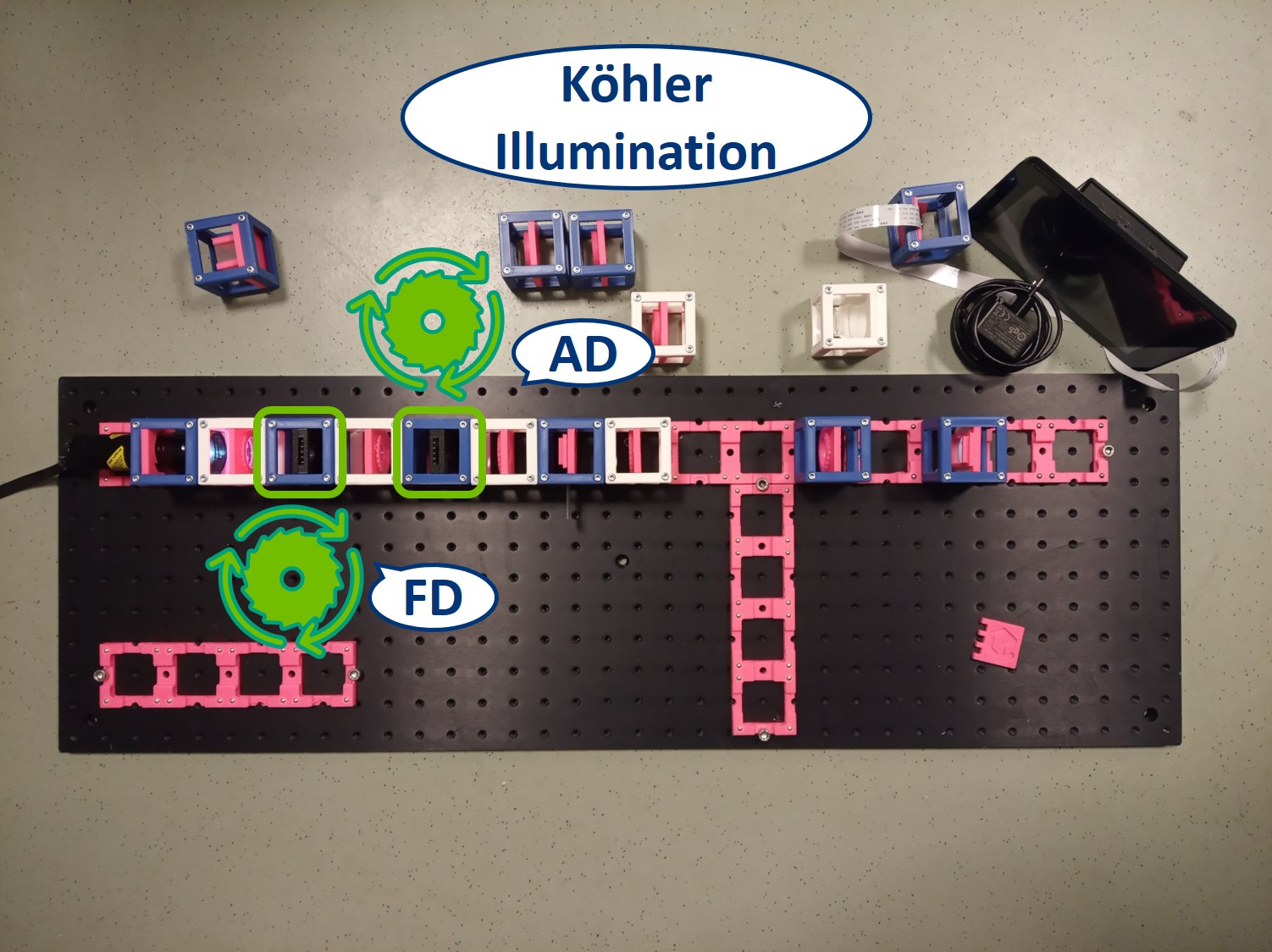
- In the Köhler illumination, the first lens after the light source is called the Collector lens. The lens between the apertures is called a Field lens. The one in front of the Sample is again the condenser lens, just as in the critical illumination.
⭐ Thanks to this configuration of three lenses, the LED is imaged on the AD and the FD is imaged on the Sample.
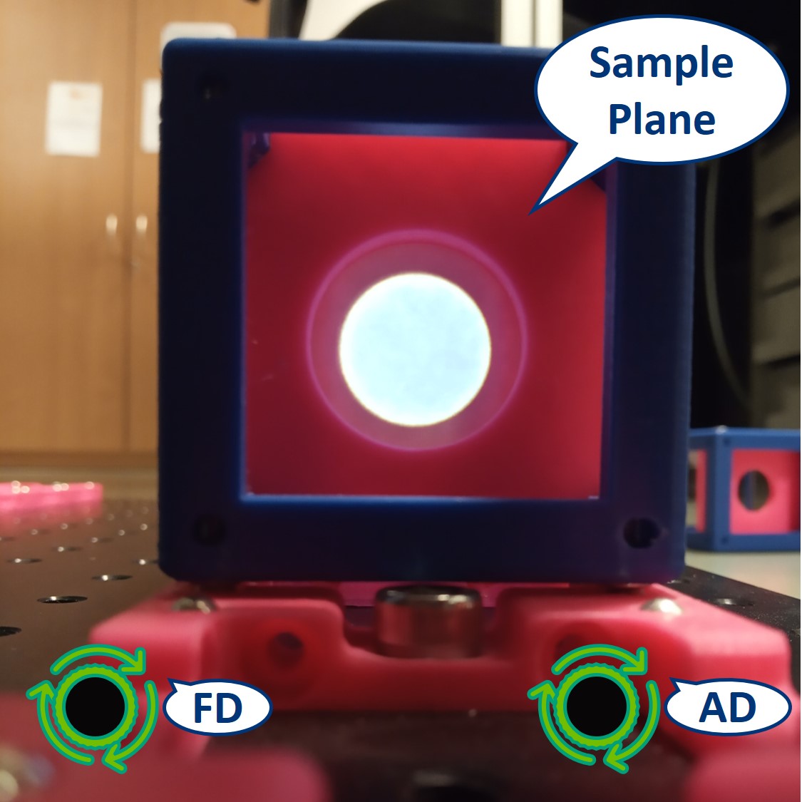
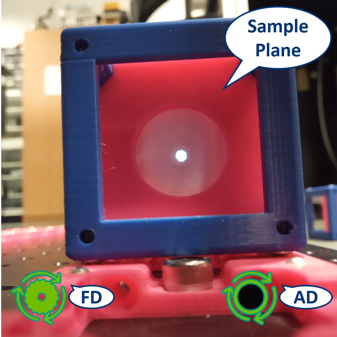
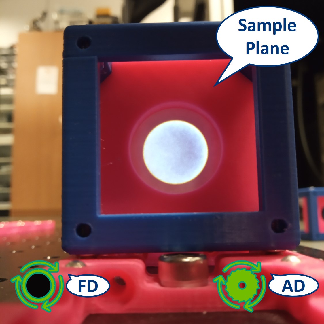
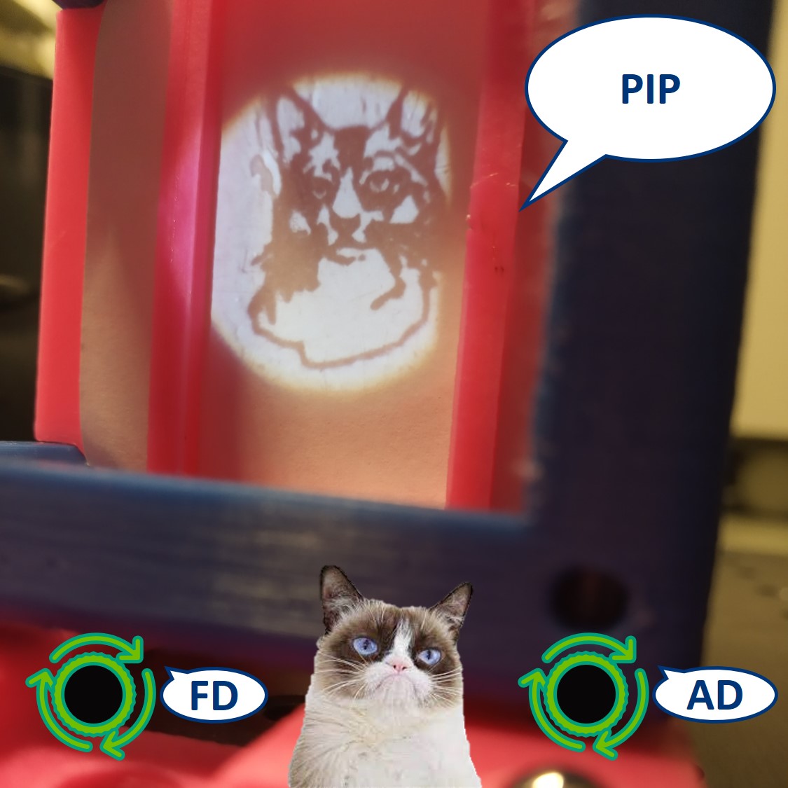
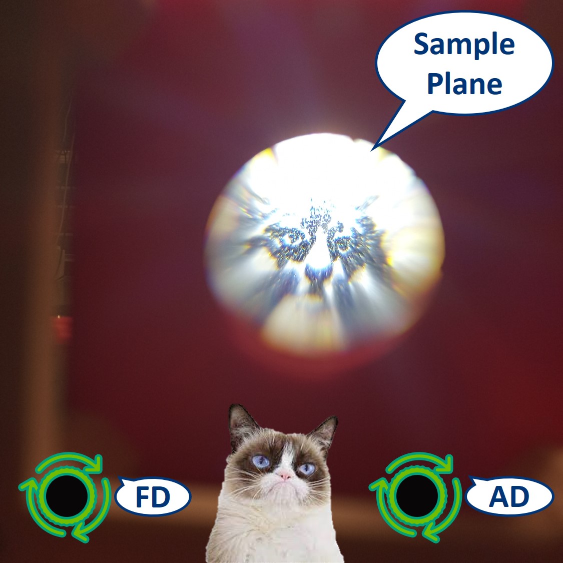
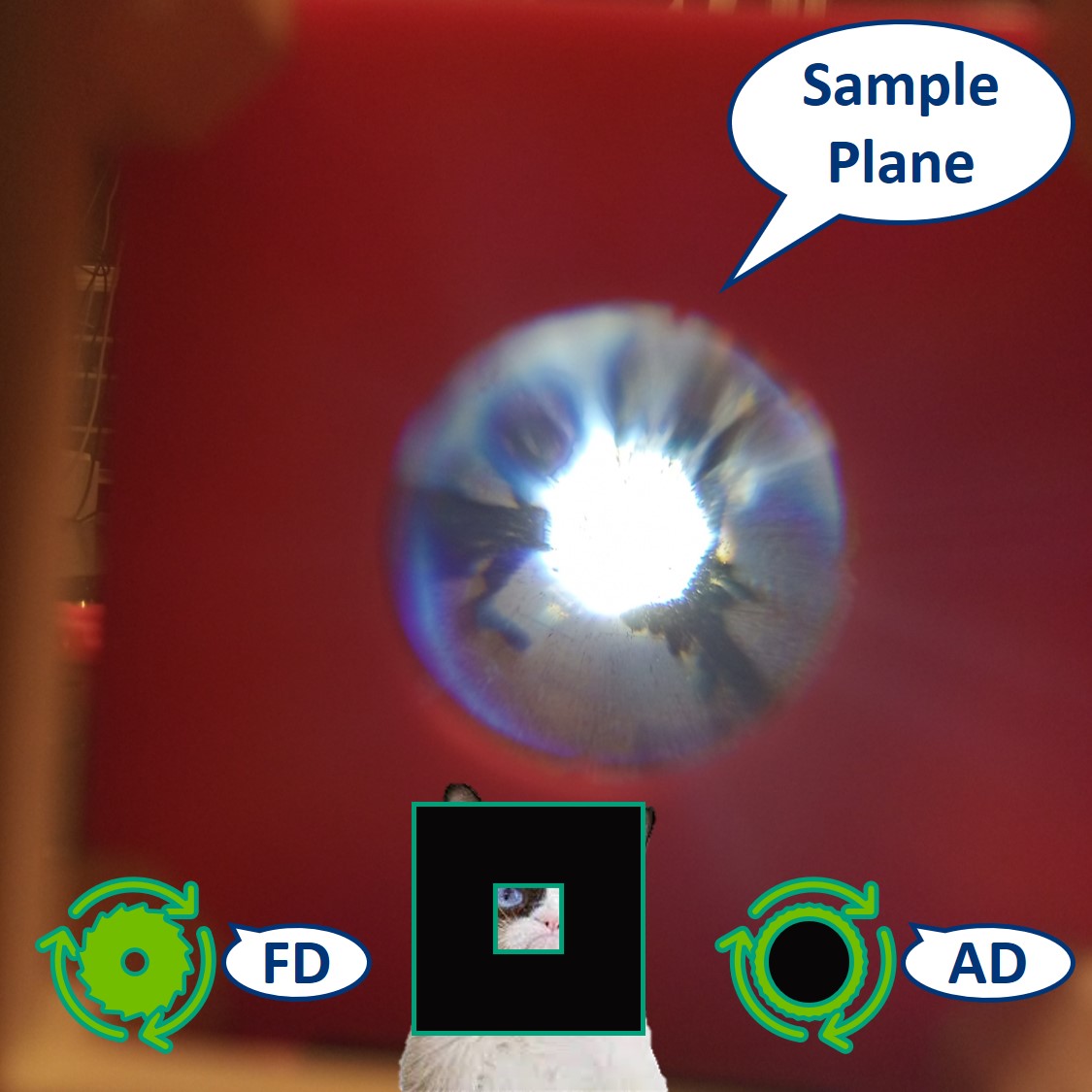
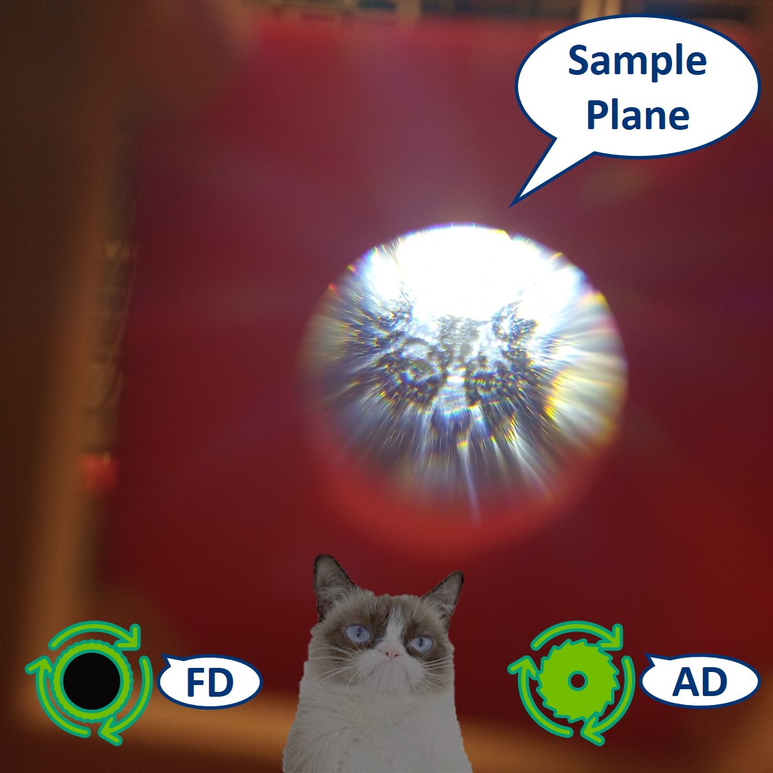
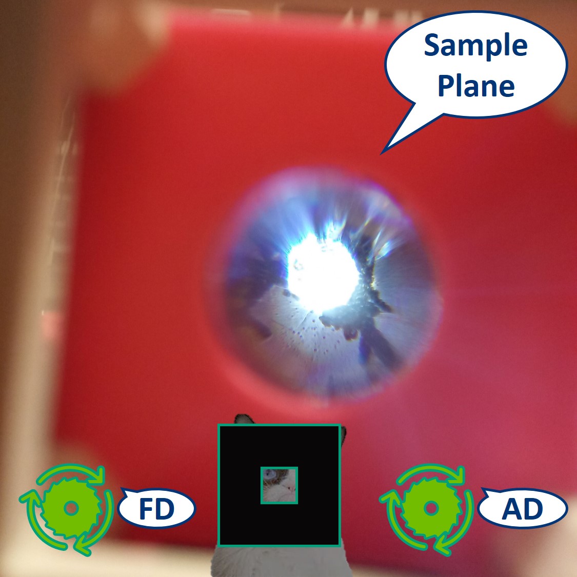
- Let's have a look at the effects of the apertures in the Sample plane. Note: because the LED is very strong, the effect of the AD is not so apparent.
⭐ In the Sample Plane: The FD is imaged on the Sample. It limits the size of the illuminated area and we can directly see the image of the FD when we close it. The AD limits the parallel light beam between the Field lens and the Condenser lens. It limits the illumination angles and therefore changes the intensity of the illumination.
Top left: both apertures open.
Top right: FD closed, AD open.
Bottom left: FD open, AD closed.
Bottom right: both apertures closed.
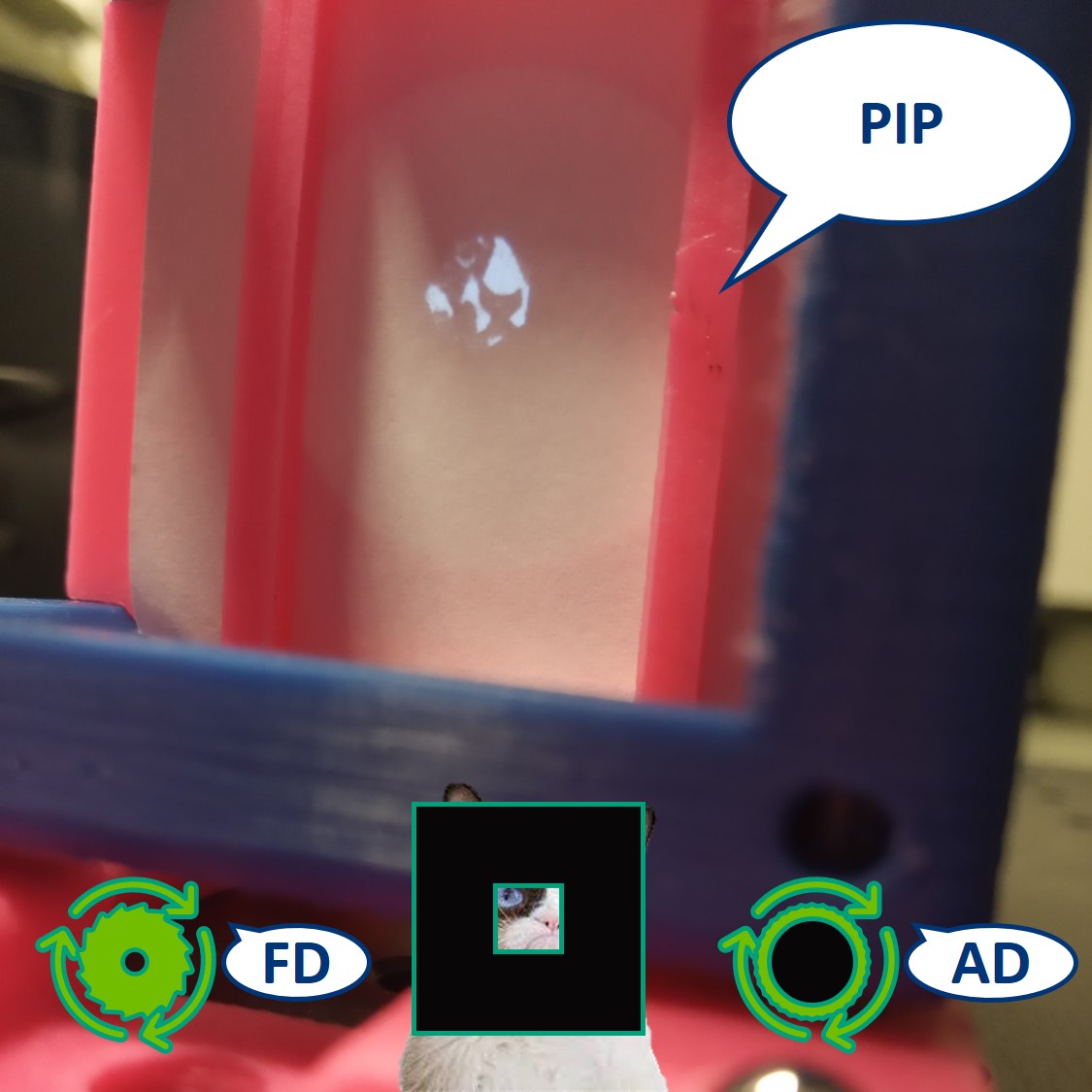
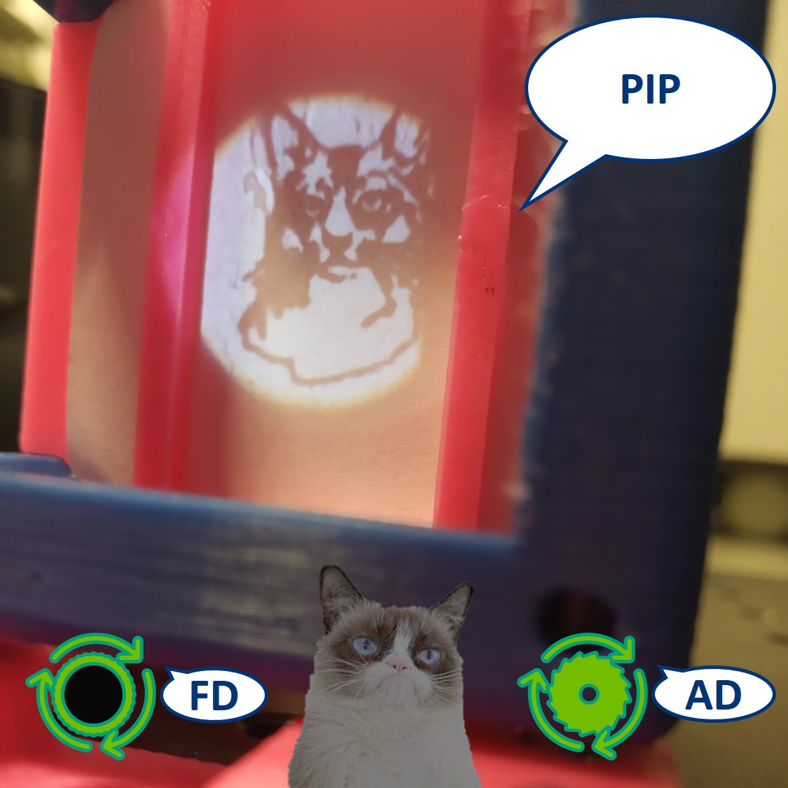
- Let's have a look at the effects of the apertures in the Primary Image Plane. Note: because the LED is very strong, the effect of the AD is not so apparent.
⭐ In the Primary Image Plane: The FD and AD have the same effect as in the Sample Plane.
Top left: both apertures open.
Top right: FD closed, AD open.
Bottom left: FD open, AD closed.
Bottom right: both apertures closed.
- Remove the screen from PIP.
⭐ Eyepiece
So far we could consider our microscope a simple one, because the image is magnified by only one system of lenses (Objective and a Tube lens together). A compound microscope uses two systems of lenses - objective and eyepiece, that multiplies (compounds) the objective. This way we can achieve higher magnification.
The magnification of an eyepiece is given by
M = 250 mm/fEyepiece ,
where 250 mm is an estimate of the "near point" distance of the eye - the closest distance at which the healthy naked eye can focus without too much strain.
The eyepiece images the PIP to the infinity, making it observable by the naked eye.
Place an eyepiece lens behind the PIP position. It is a single plano-convex lens with f' = 50 mm.
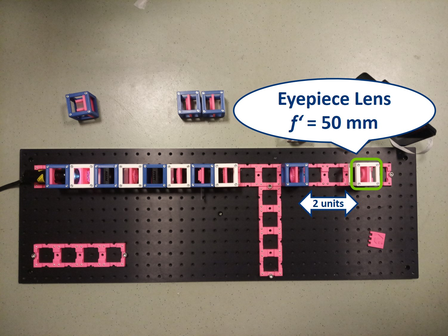
Careful! Put a lens tissue in front of the flashlight to dim it before you look into the strong light. Then look through the eyepiece lens. Note: because the LED is very strong, the effect of the AD is not so apparent.
⭐ With the eyepiece we observe the Sample Plane imaged on the PIP. The diaphragms will have the same effect as we observed in the previous steps.
Top left: both apertures open.
Top right: FD closed, AD open. Here we see the issue caused by the super bright light source - we should see the image only in the very bright region and not around it.
Bottom left: FD open, AD closed.
Bottom right: both apertures closed. Here we see the issue caused by the super bright light source - we should see the image only in the very bright region and not around it.
⭐ Note that you cannot put your eye anywhere behind the eyepiece. To maximize the field of view, your iris (the pupil of the eye) must match the so-called Ramsden disc. This is the smallest diameter of the light beam coming from the eyepiece. You can find it using a piece of paper and tracing the Light that emerges from the eyepiece. The smallest spot is roughly in the focal plane of the eyepiece (If your microscope is properly aligned).
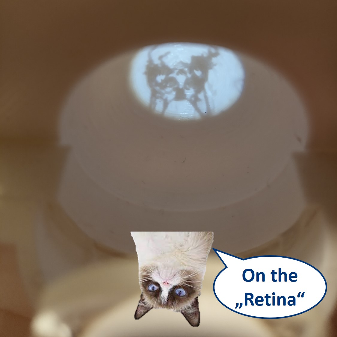
Place the Eye Cube behind the eyepiece. On the back of the "Eye" you can see the image similarly as it's formed on your retina.
This is an aligned compound infinity-corrected microscope with proper Köhler illumination.
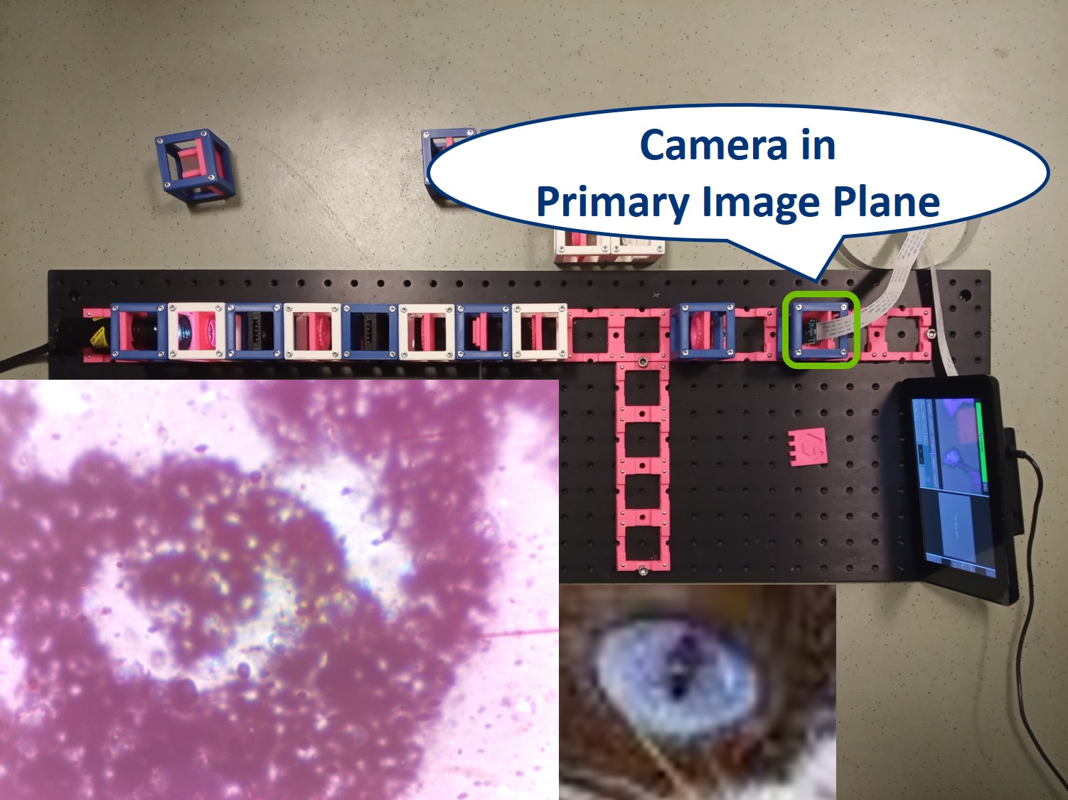
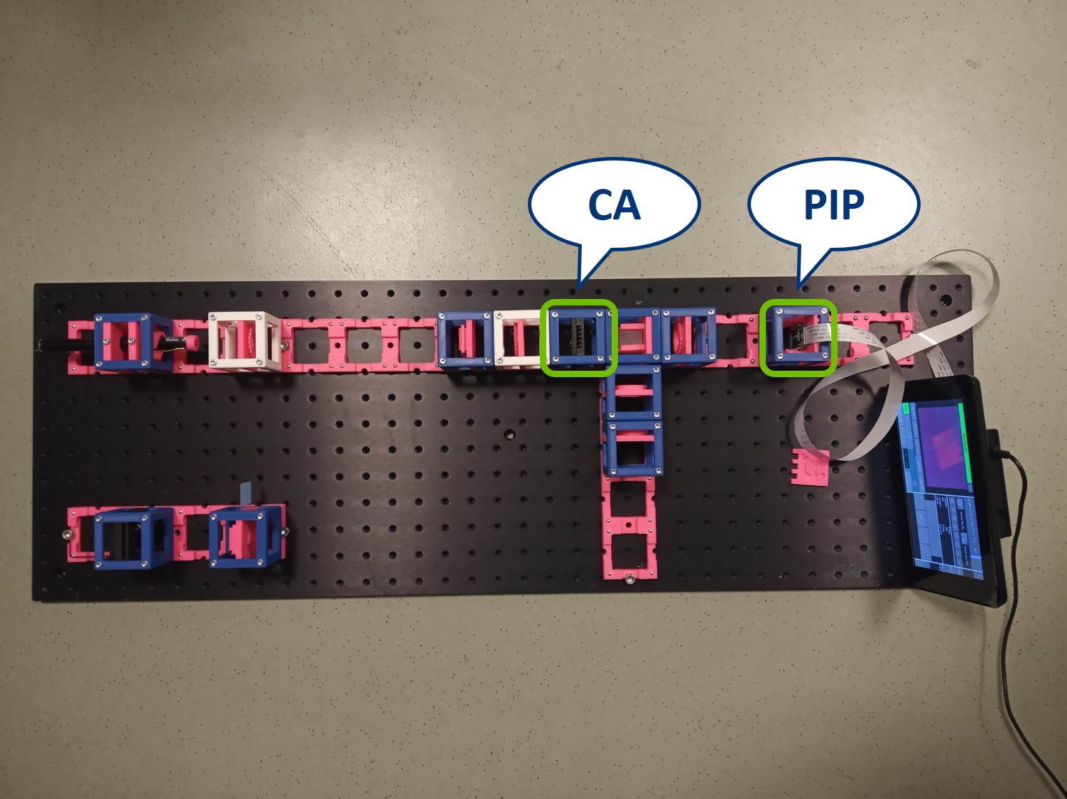
Place the RasPi Camera in the PIP and switch on the UC2-GUI on the RasPi. The field of view of the camera is much smaller than the one of the eye or with the paper screen. Align the camera to see a sharp image (II. Focussing Trick).
⭐ Field set and Aperture set of conjugate planes
In any imaging system there are two important sets of planes: Field set, containing the images of the object and the Field diaphragm and Aperture set, containing the images of the light source and the Aperture diaphragm. Those two sets are mathematically related to each other by Fourier transform. Both sets therefore contain all the information of the image and the image can be manipulated in either of them.
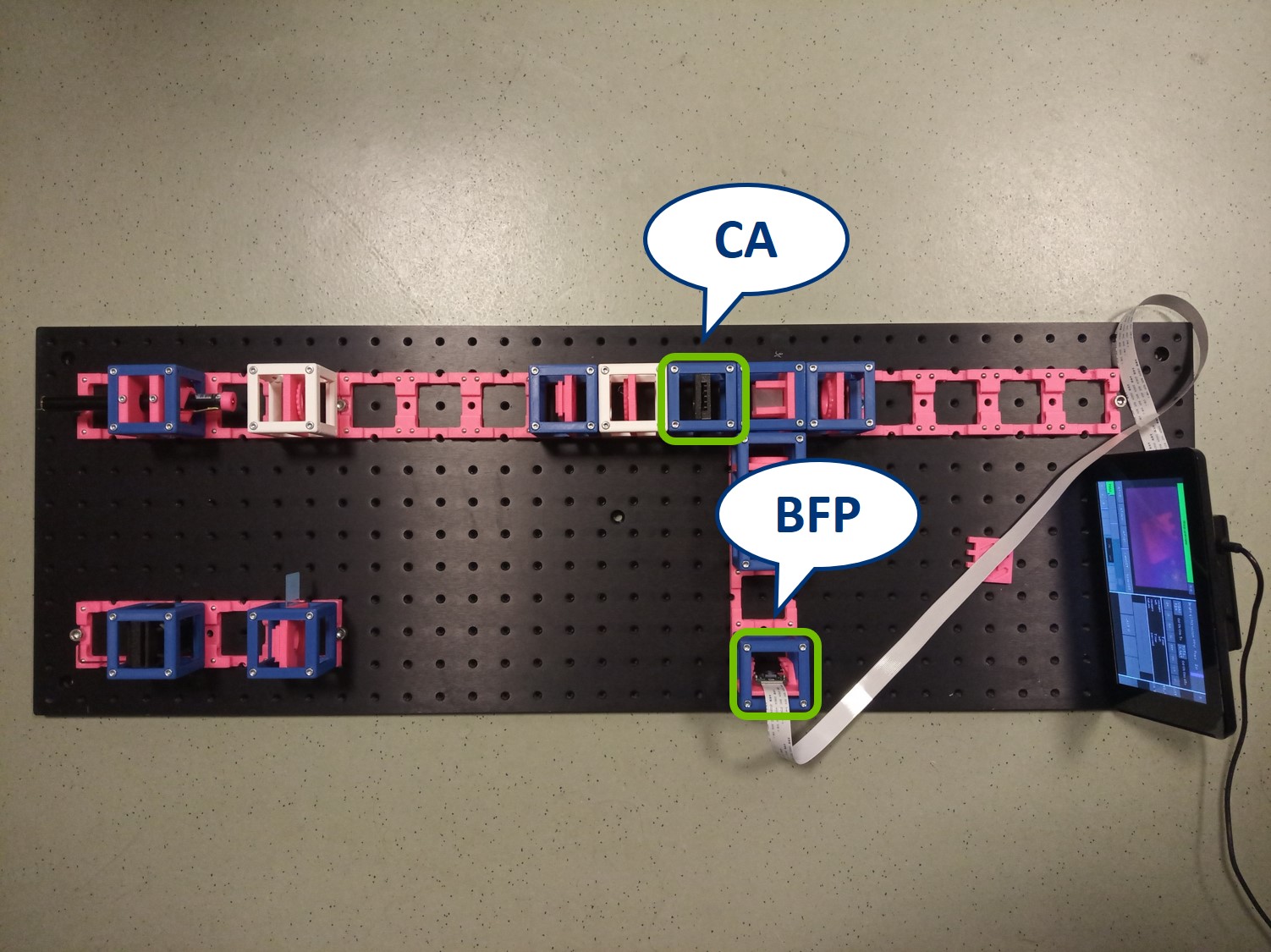
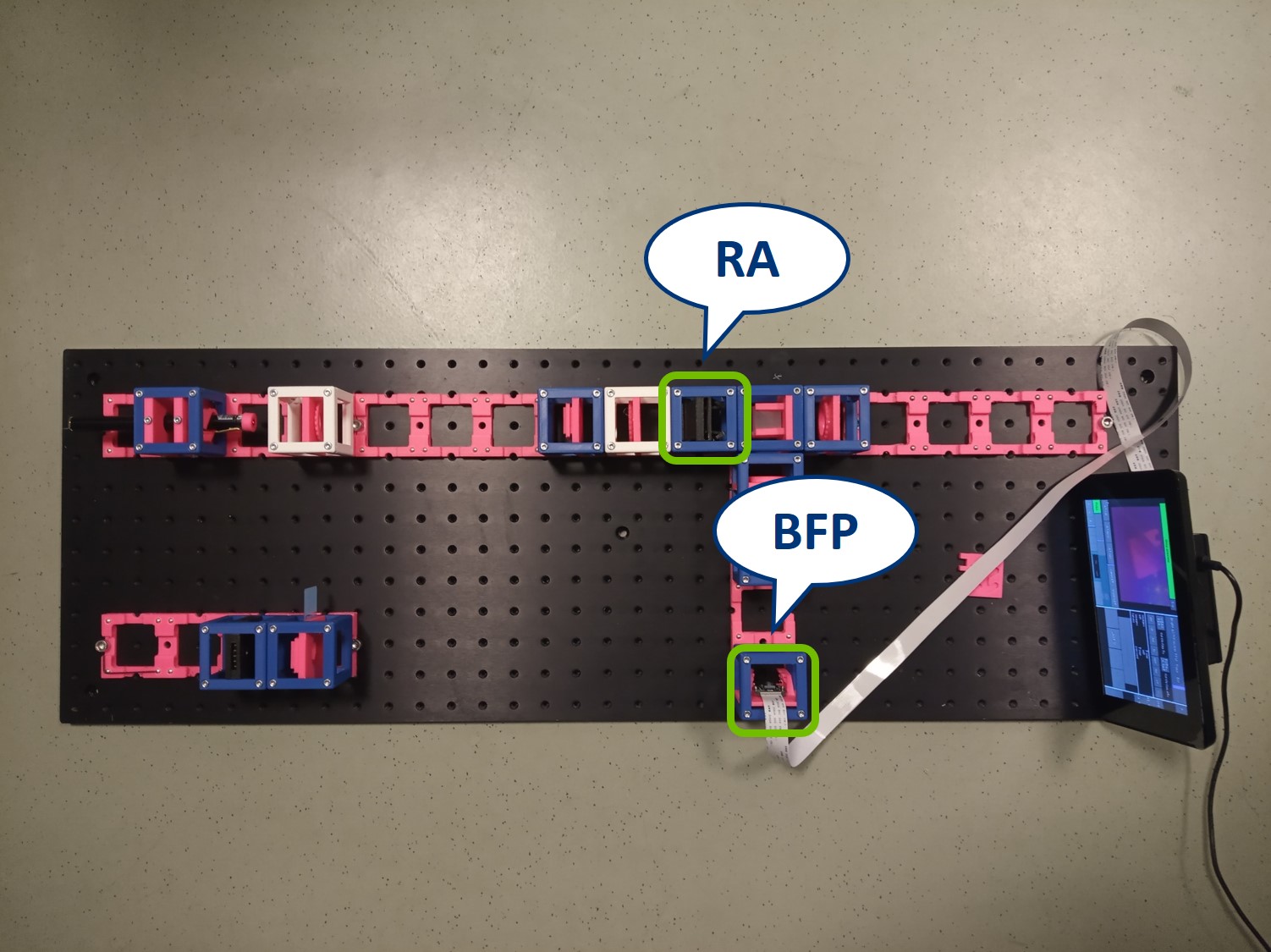
In order to observe both sets of planes simultaneously, we can build a side arm and image the BFP there.
The Aperture set of conjugate planes: Lamp filament, Aperture diaphragm, Back Focal Plane of the objective, Exit pupil of the eye. The BFP will be imaged in the side arm.
Because we've build our system entirely of infinite conjugates, each pair of lenses is imaging whatever is in the front focal plan of the first one in the back focal plane of the second one. Thanks to this, we have access to all the conjugate planes and we can easily manipulate them.
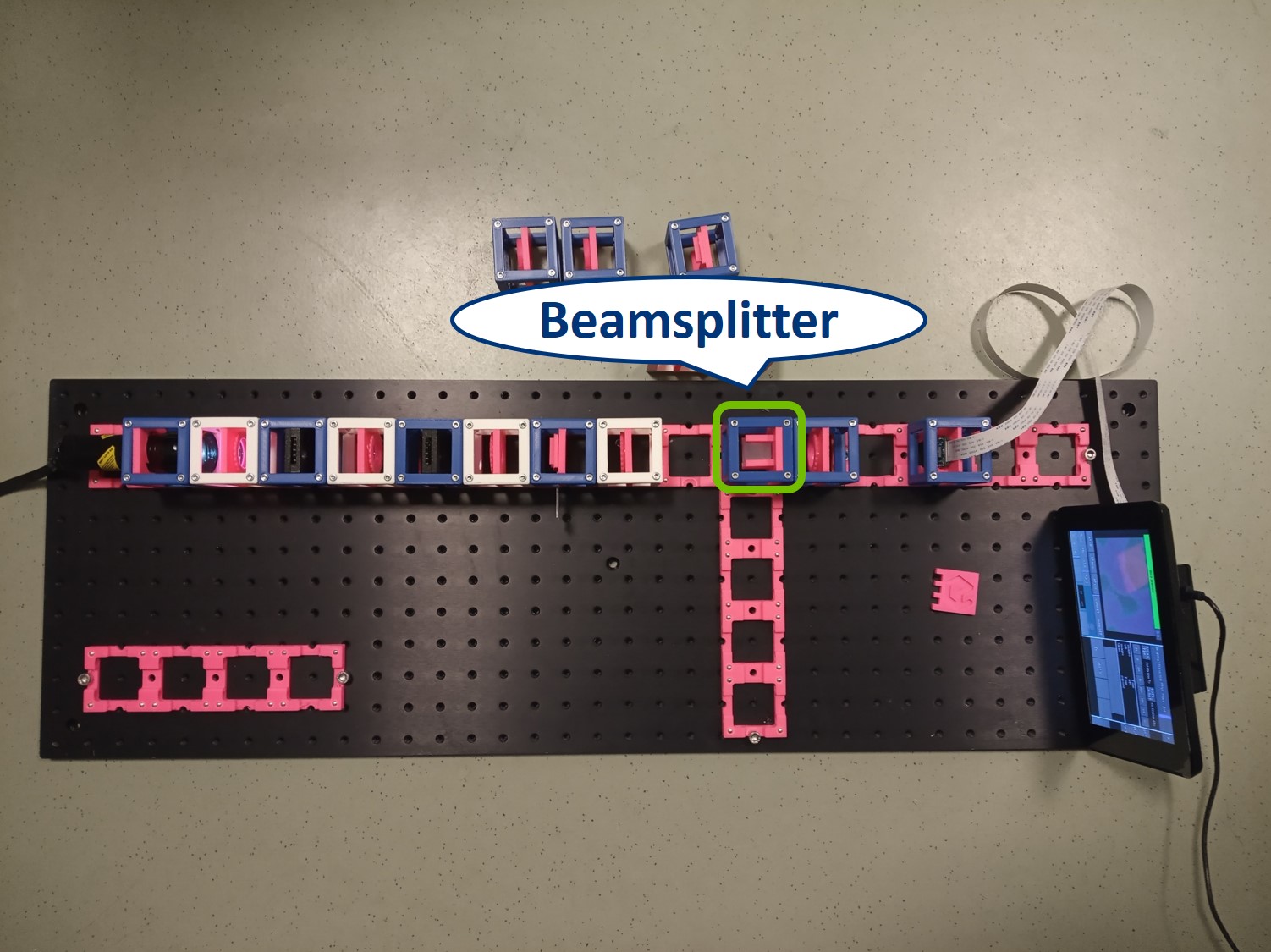
Building the side arm: Place the Beamsplitter Cube. It has to be oriented in such a way that it will reflect half of the incoming light in the direction of the side arm. The rest of the incoming light is still transmitted to the PIP.
Place the first relay lens next to the Beamsplitter, in the side arm. It is a single plano-convex lens with f' = 100 mm.
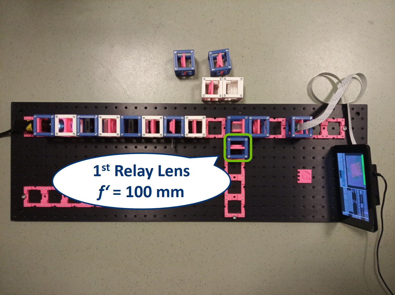
Place the second relay lens behind the first one, in the side arm. It is also a single plano-convex lens with f' = 100 mm.
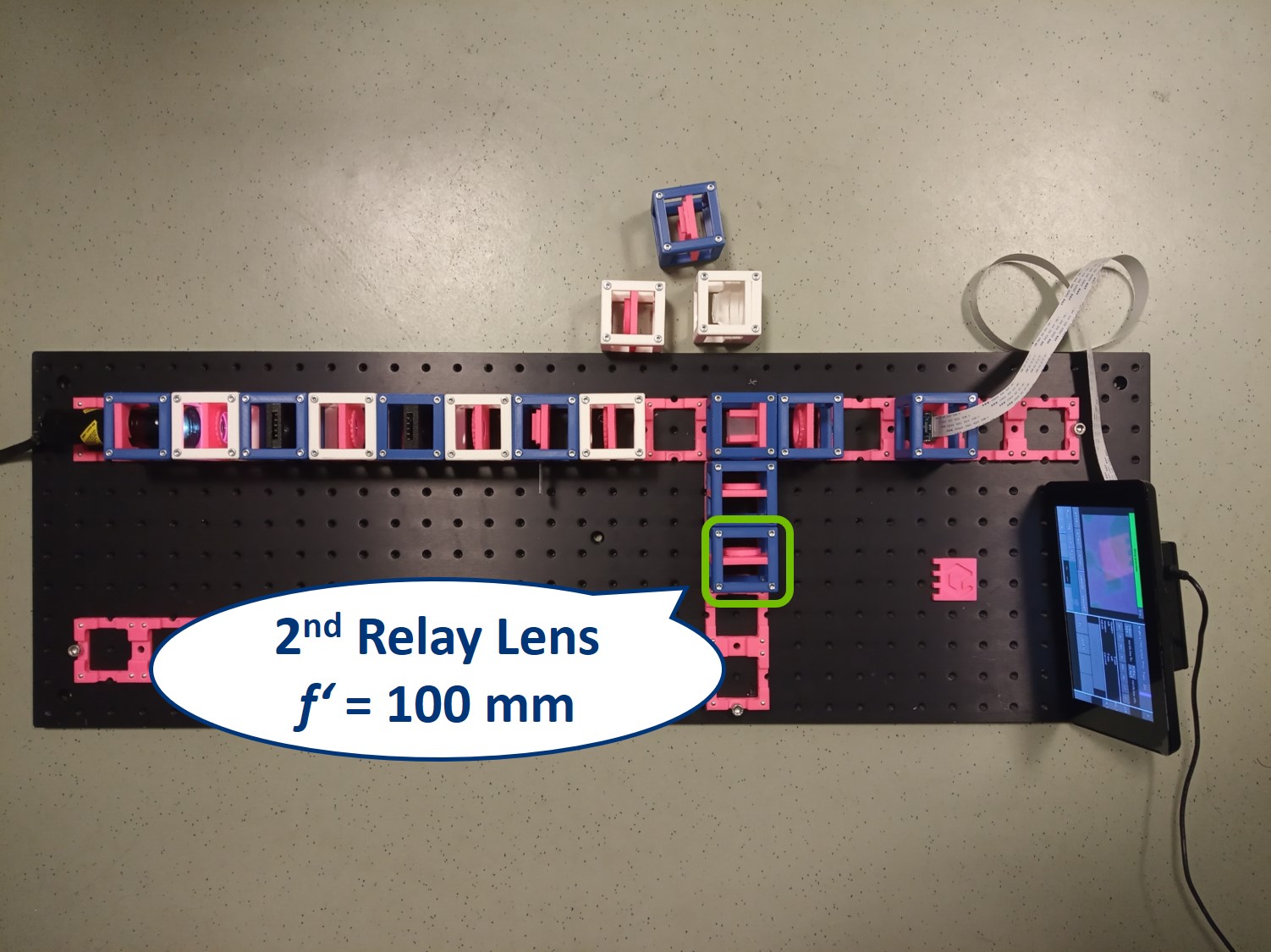
⭐ We build another infinite conjugate system in the side arm and its magnification is again given by M = - f2/f1 . Because both of the relay lenses have the same focal length (100 mm), the magnification in the side arm is equal to -1. We can see an inverted image of the BFP, in the same size as in the actual Back Focal Plane of the Objective.
Place the paper screen in the focal plane of the second relay lens. This is where you image the back focal plane of your objective.
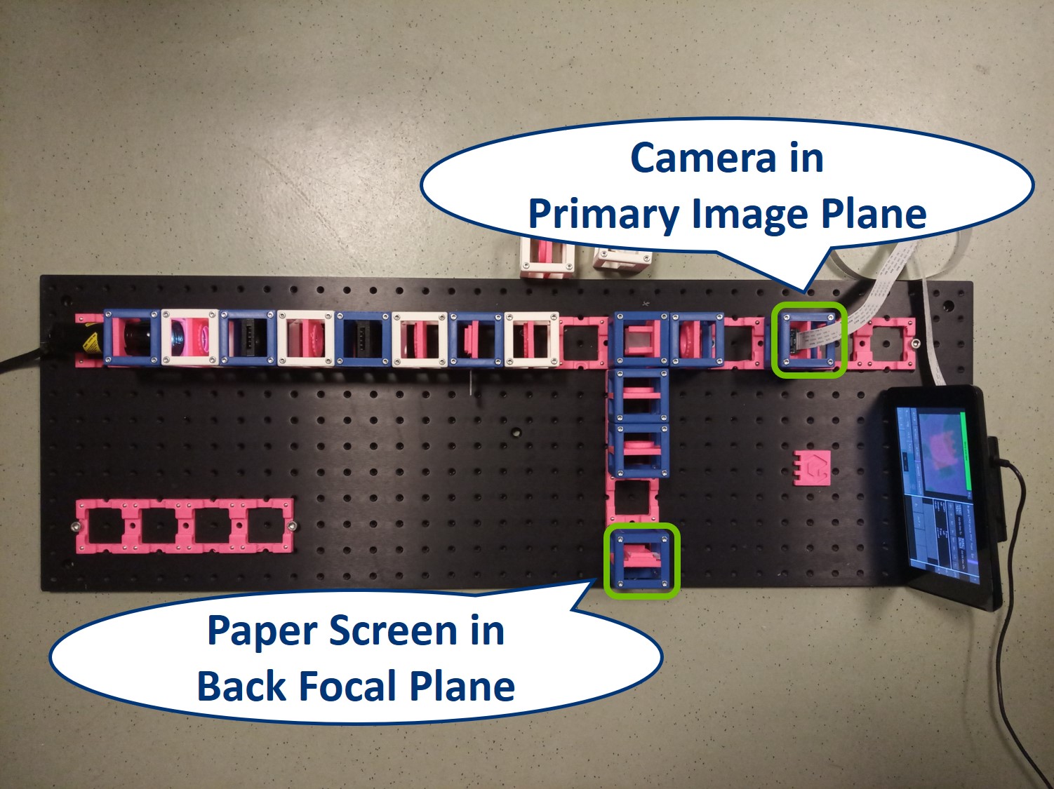
Let's have a look in the BFP, as it's imaged in the side arm.
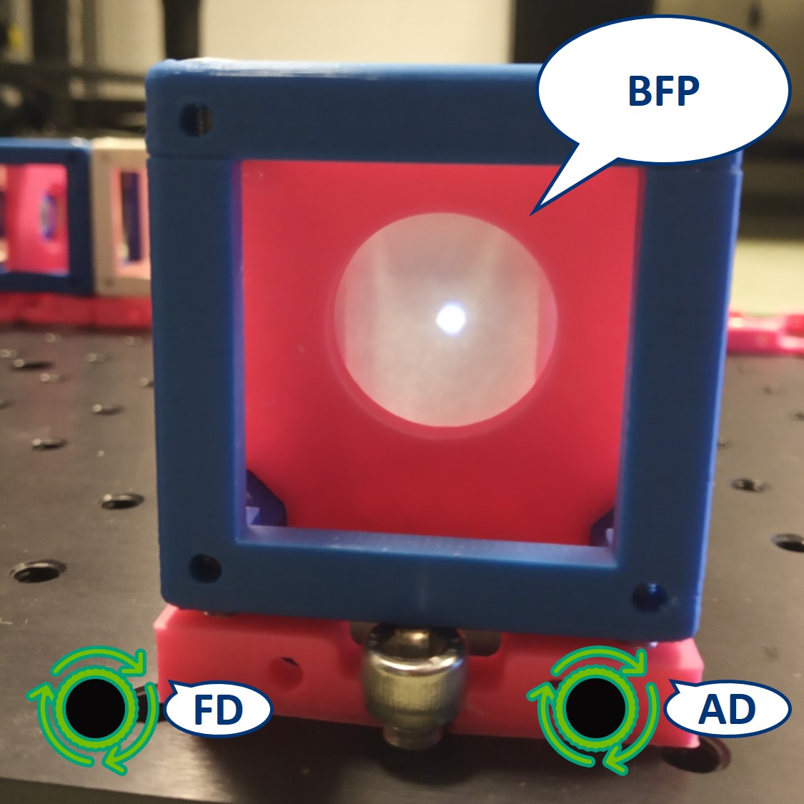
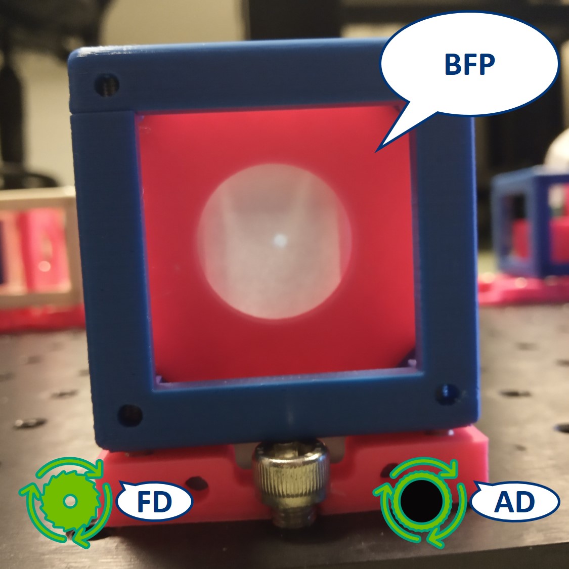
⭐ In the BFP the apertures have the opposite effect as in the PIP. The AD is imaged into this plane while the FD limits the angles of the illuminating rays. We also see an image of the LED in the BFP.
Top left: both apertures open.
Top right: FD closed, AD open. The image is dimmer.
Bottom left: FD open, AD closed. The illuminated area is smaller.
Bottom right: both apertures closed.
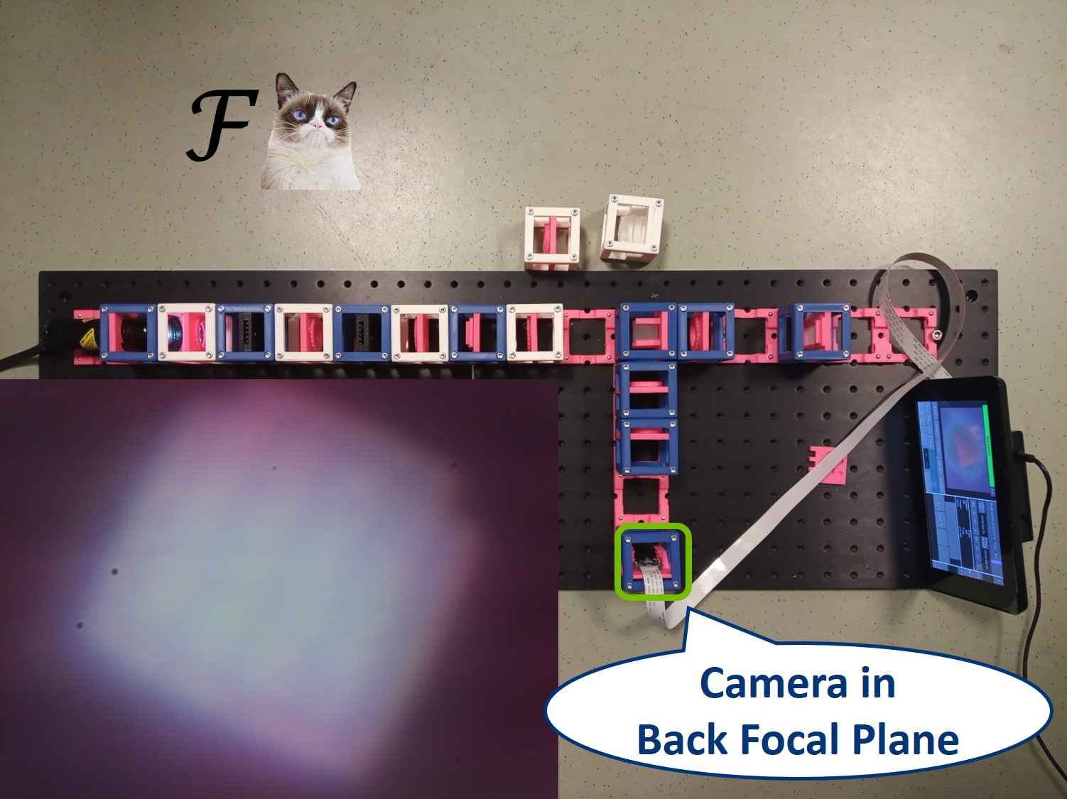
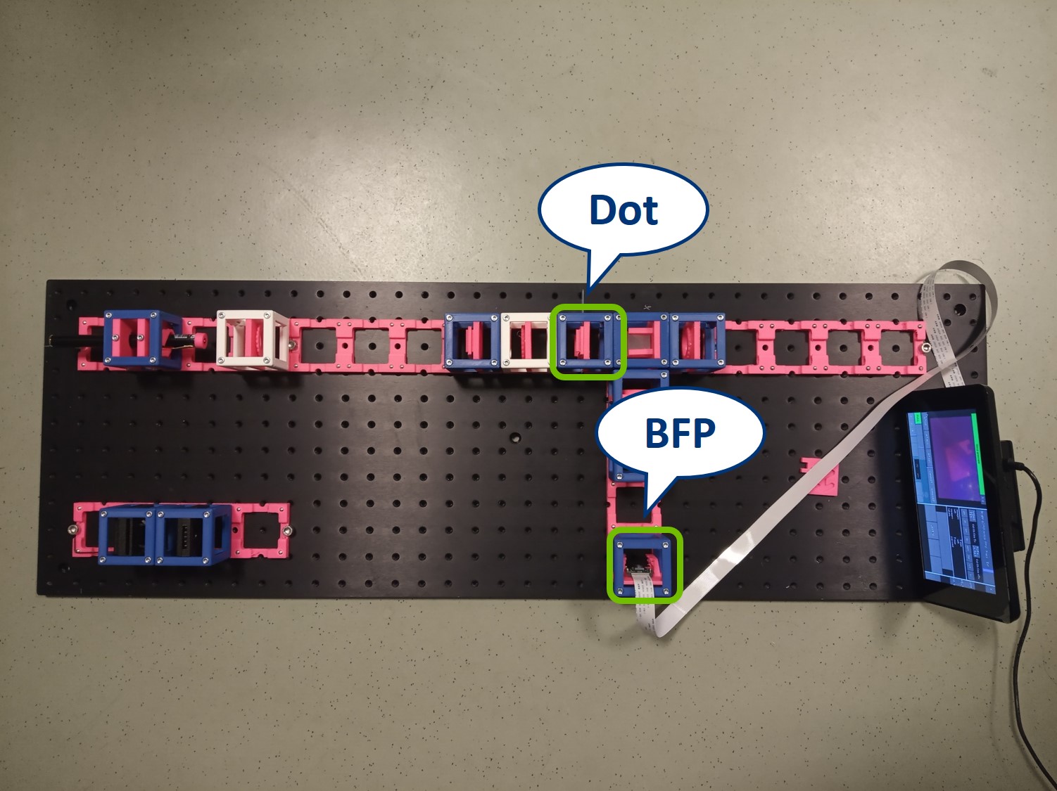
- Switch the camera with the paper screen, so we can see the BFP on the RasPi. We could see the Fourier transform of our cat there but because of the high intensity of the flashlight, we only see the image of the LED.
⭐ The magnification of the LED image formed here is given by the multiplication of the magnifications of al the infinite conjugate systems that are imaging it. It is given by MLED in BFP = - fField lens/fCollector × fObjective/fCondenser × fRelay lens 2/fRelay lens 1 . Because each pair of the lenses has actually the same focal length, the magnification of the LED in the BFP is -1 and we see an inverted non-magnified image of it.
- This is the complete first experiment: Compound Microscope with Köhler Illumination and access to all the conjugate planes. You would be able to demonstrate the Abbe Diffraction Experiment with this as well but it's much nicer with the setup we will build now.
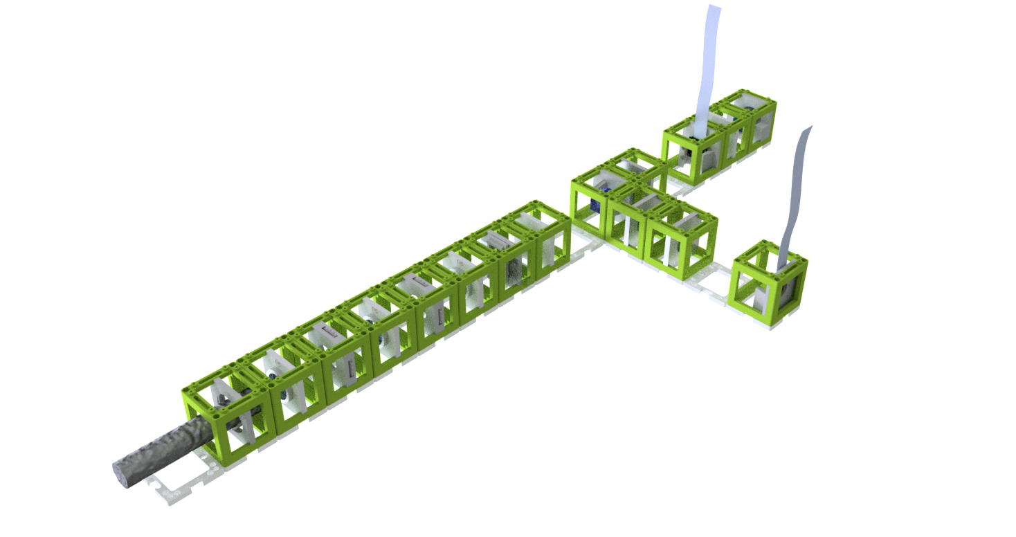
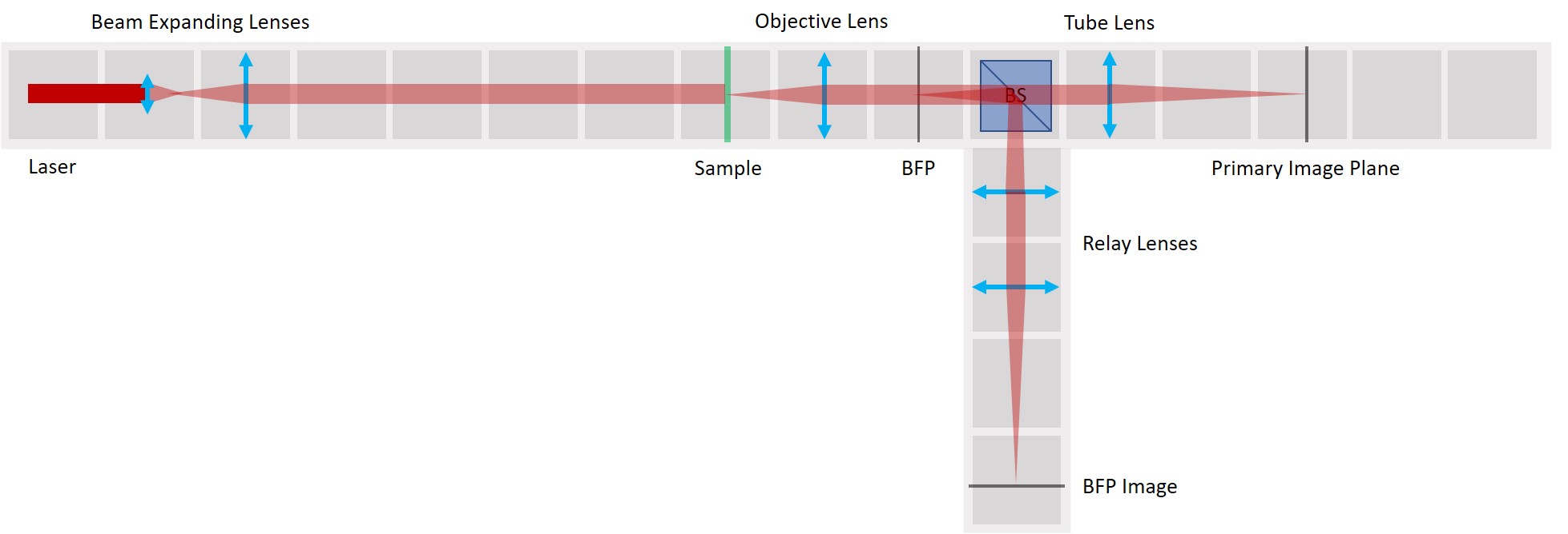
Abbe Diffraction experiment
⭐ Abbe Diffraction experiment
Until Ernst Abbe and Carl Zeiss teamed up in 1866, microscopes were produced by the trial and error method. Abbe discovered after many calculations and experiments that the diffraction image in the Back Focal Plane of the objective is essential for image formation. We're going to explain his findings during the demonstration of his famous experiment.
We use a laser pointer as a light source and expand it using two lenses. The imaging path is the same as in the microscope in the first experiment and therefore we can observe the image of our sample in the main arm and the image of the BFP in the side arm.
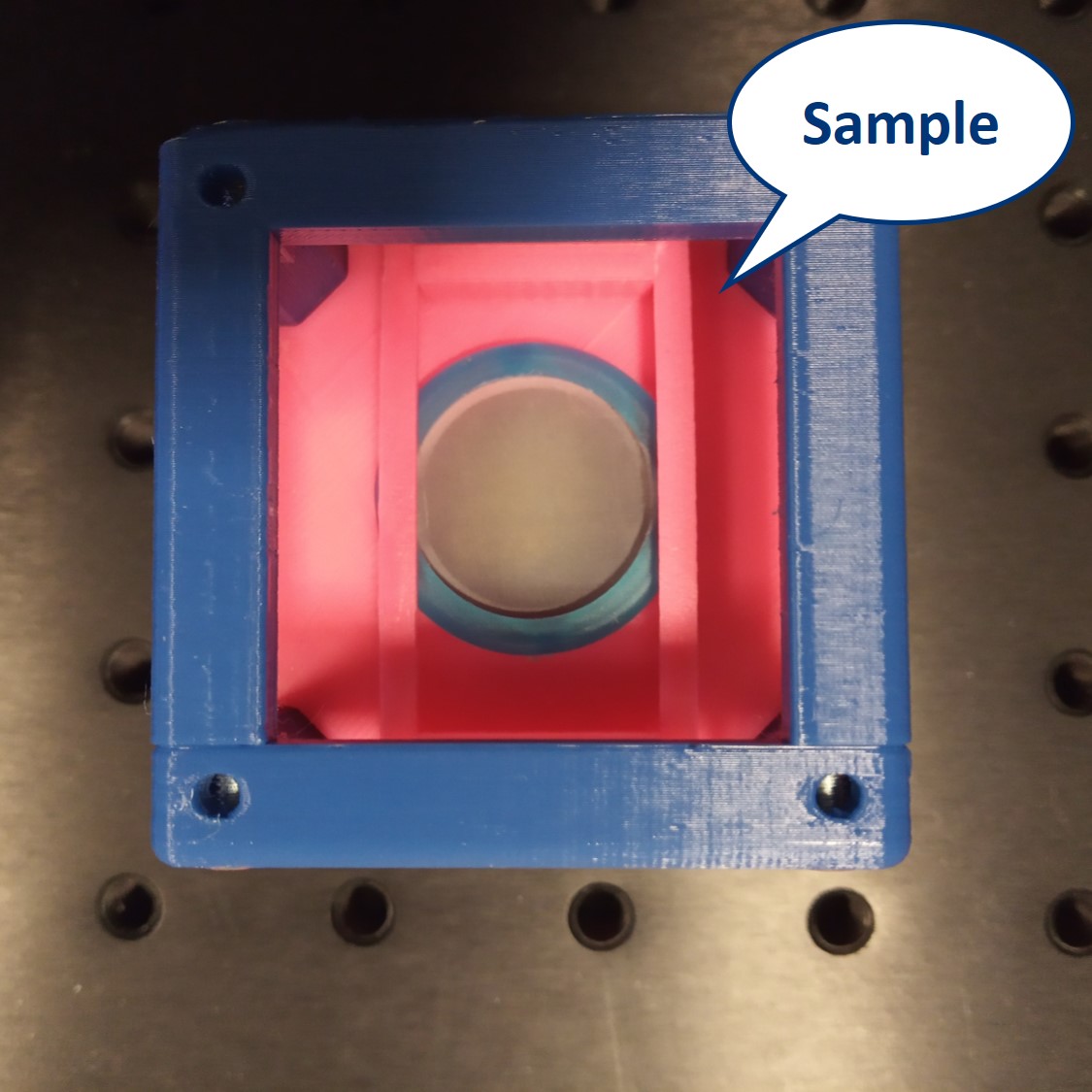
We use a very fine fish net as a sample here. You could try a net like this one. Another idea is to try one of these plastic tea bags. Or a diffraction grating.
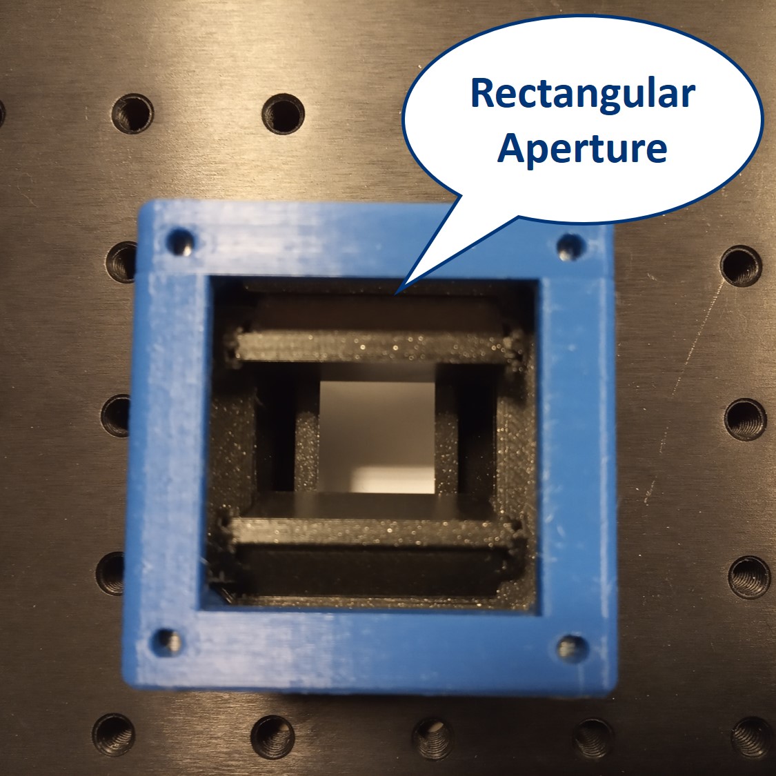
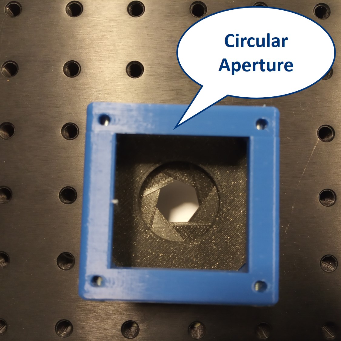
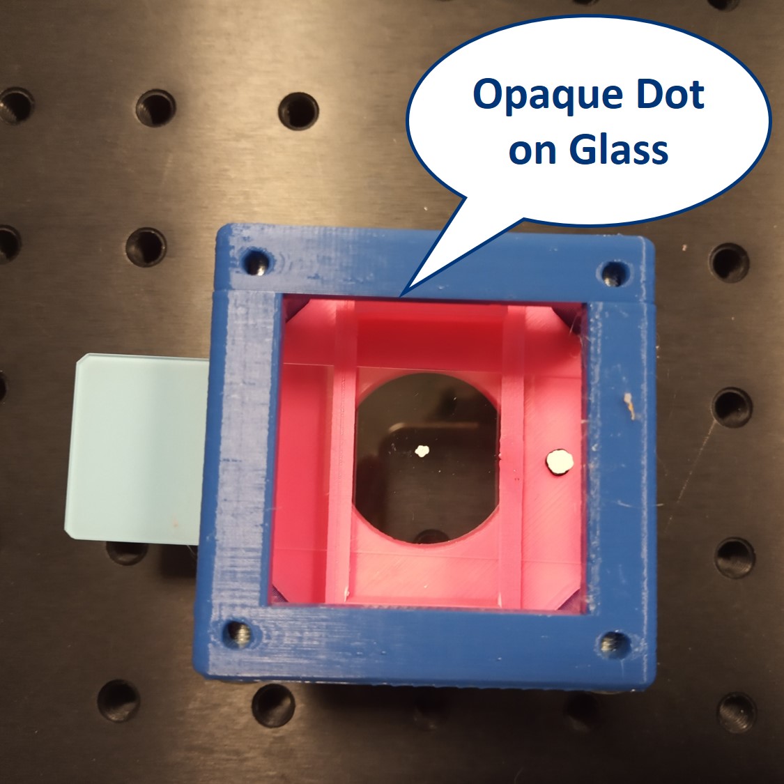
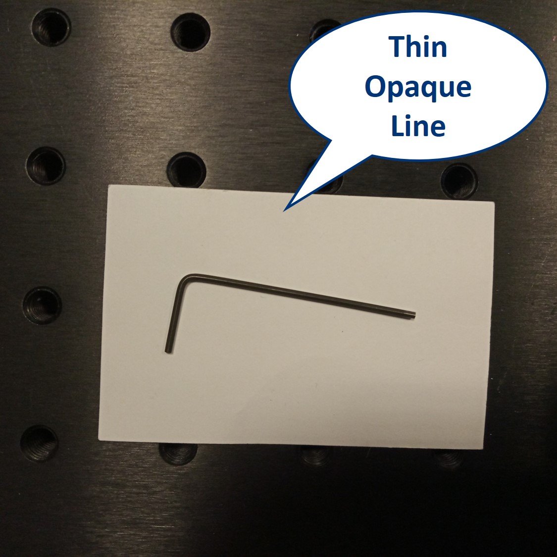
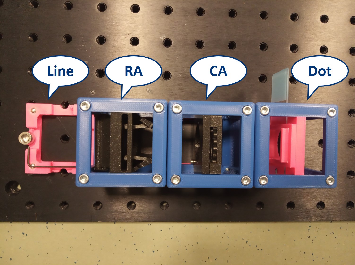
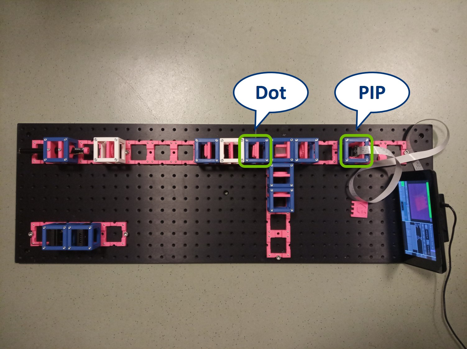
We provide a circular aperture and a rectangular aperture to be used in the BFP. We also suggest to use an opaque dot (a small dot made with some marker or pain on a microscope slide) and a thin line object (like this tiny hex key here). The apertures block the light from the outside while the dot and line can block the center of the light path.
As mentioned earlier, we keep the imaging path in both main arm and side arm. Remove the illumination part of the microscope and also the Eyepiece.
Besides the apertures that we already prepared, we will need :
- Laser Cube with laser pointer (1)
- 1× Lens Cube with 50 mm lens (2)
For now, place the camera in PIP.
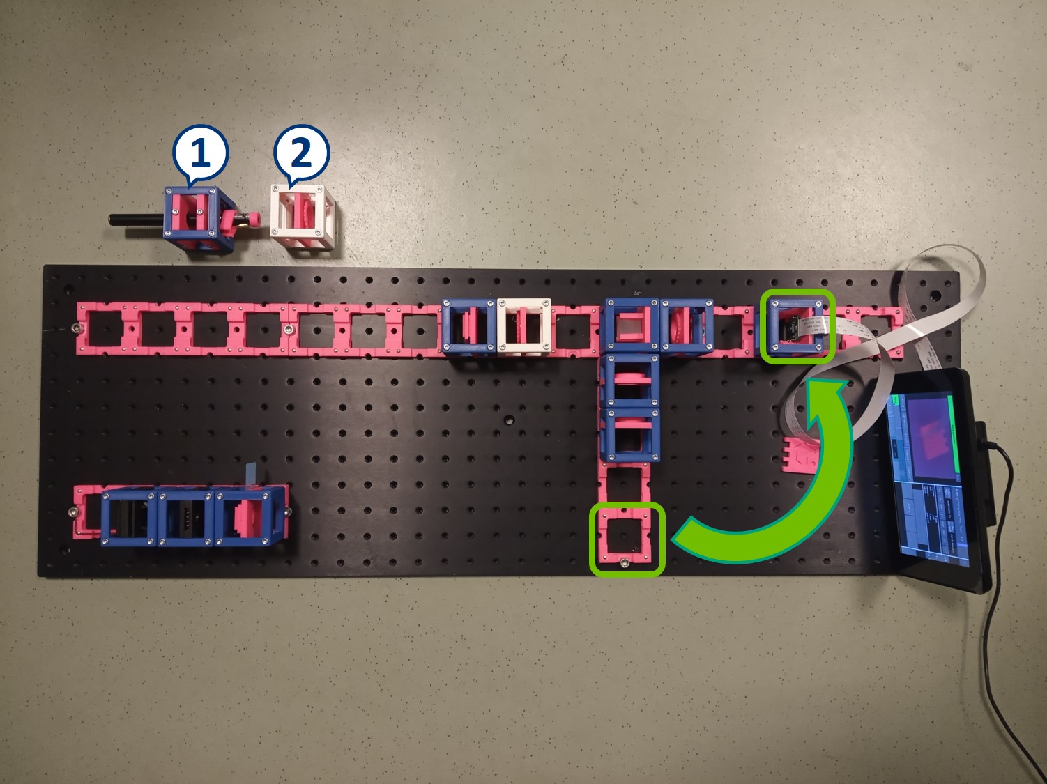
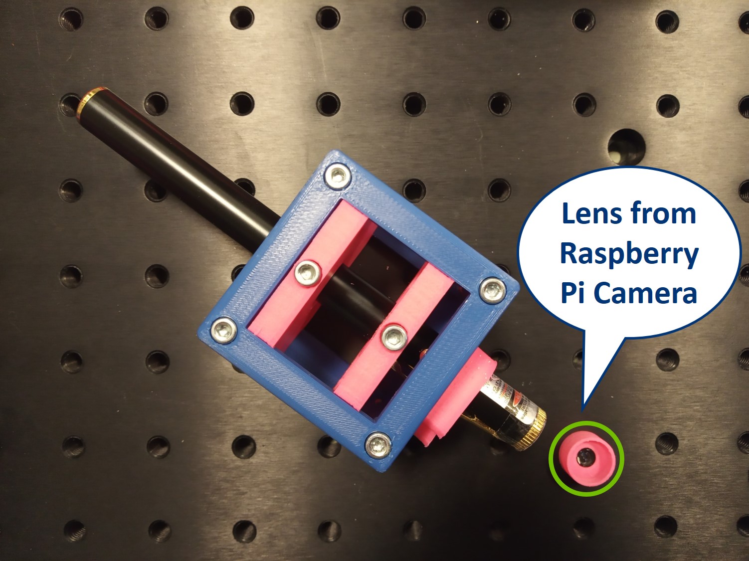
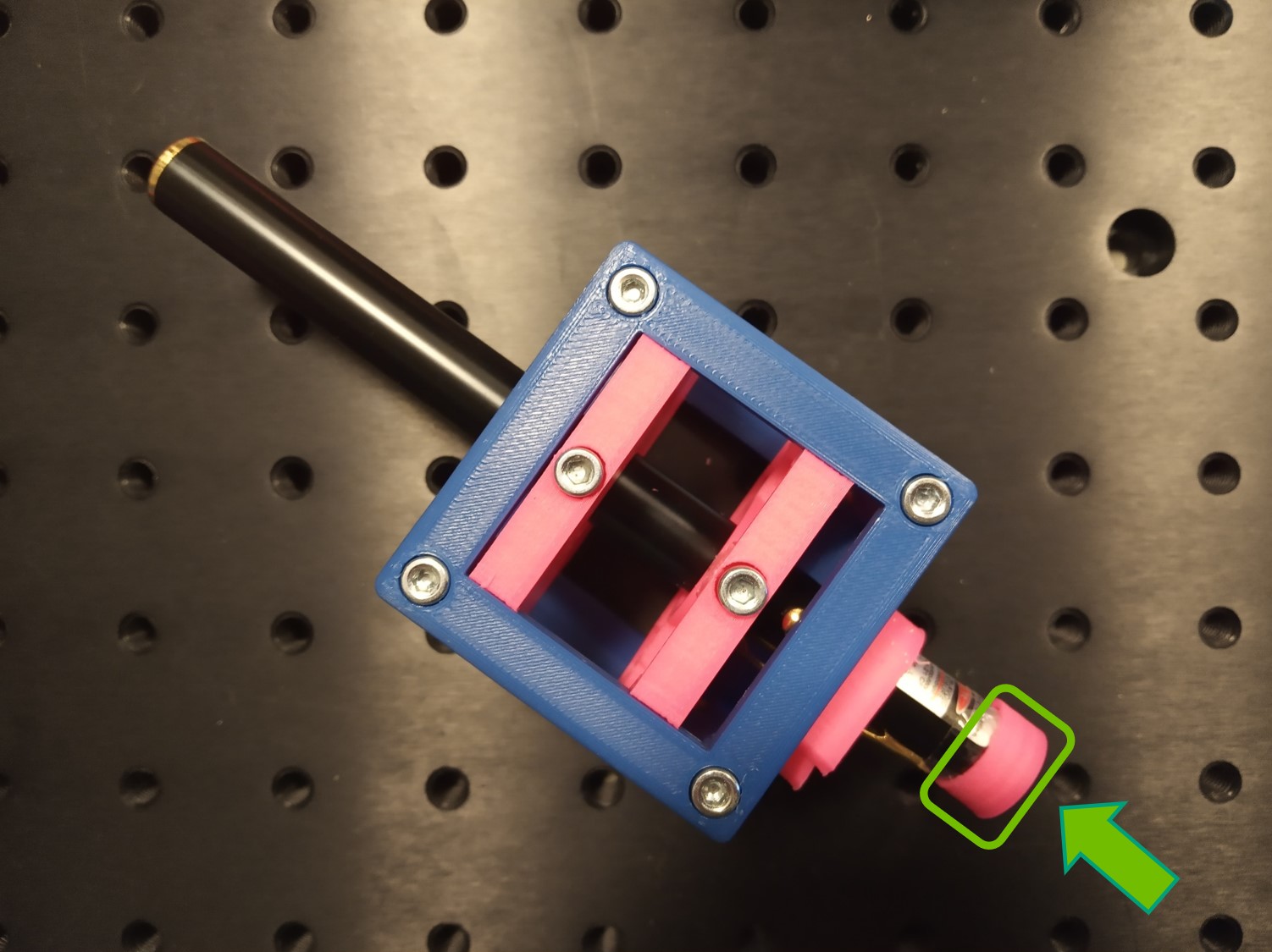
- The laser is equipped with a cap that holds a lens from the RasPi camera. Make sure to put it on, otherwise you won't be able to create an expanded parallel beam.
- Place the Laser cube on the baseplate as shown in the picture.
Careful! Do not hit anybody's eyes with the laser beam. Keep the laser off if you're not using it at the moment. Always point the laser away from people. Block the light if it's leaving the table you're working on.
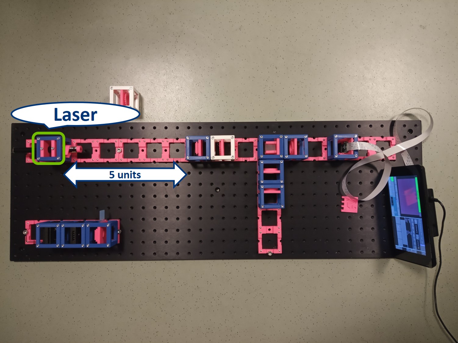
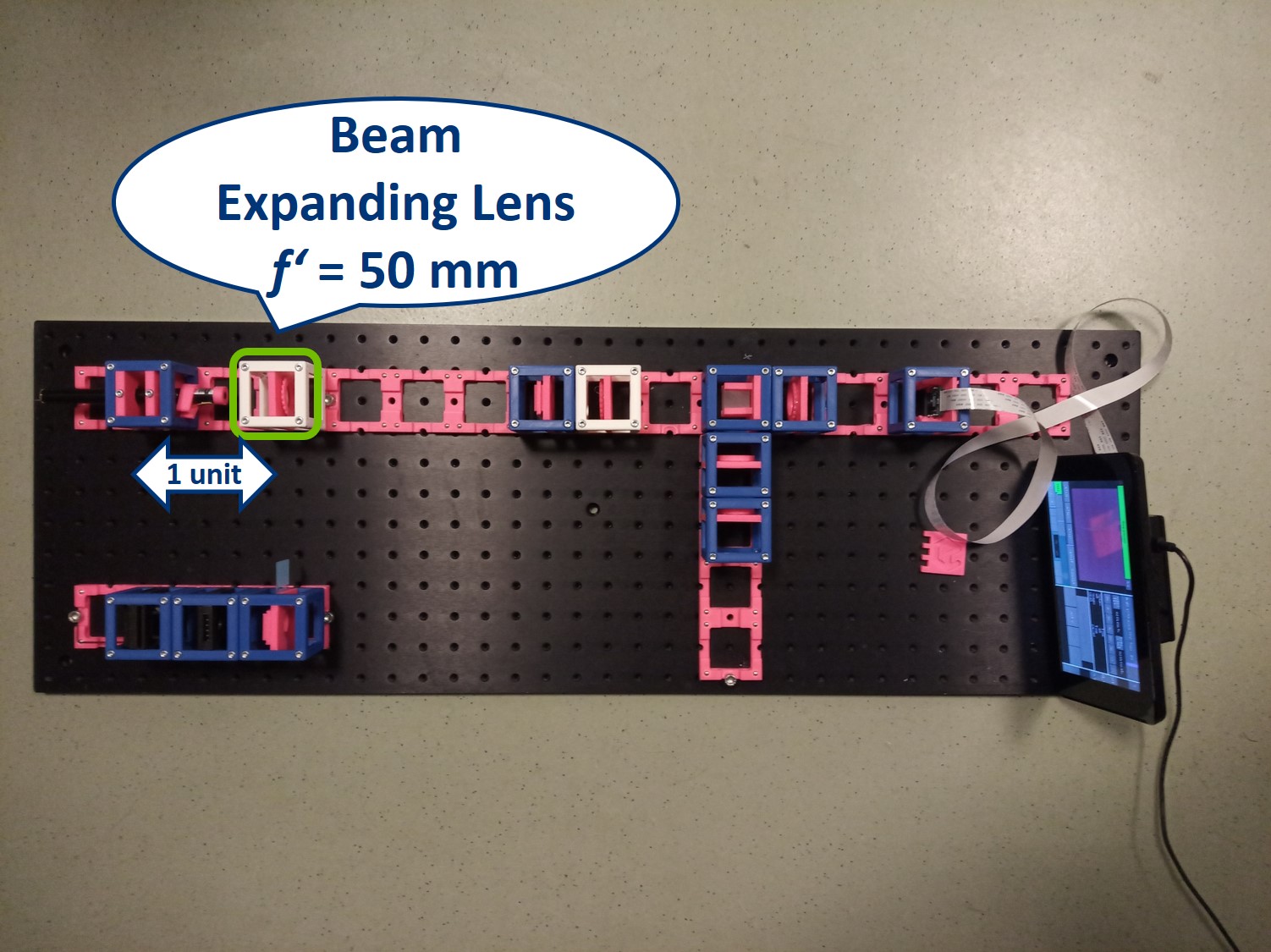
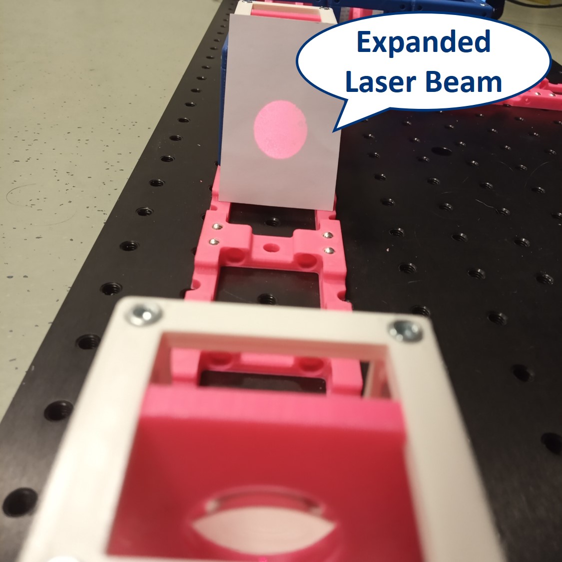
Place the lens for beam expansion behind the Laser cube as shown in the picture. It is a single plano-convex lens with f' = 50 mm. Align the lens to illuminate your Sample with a collimated beam - the diameter of the beam should be the same just after the lens cube and also far away from it. When you beam is well-collimated, the distance between the laser+lens duo and the Sample doesn't matter.
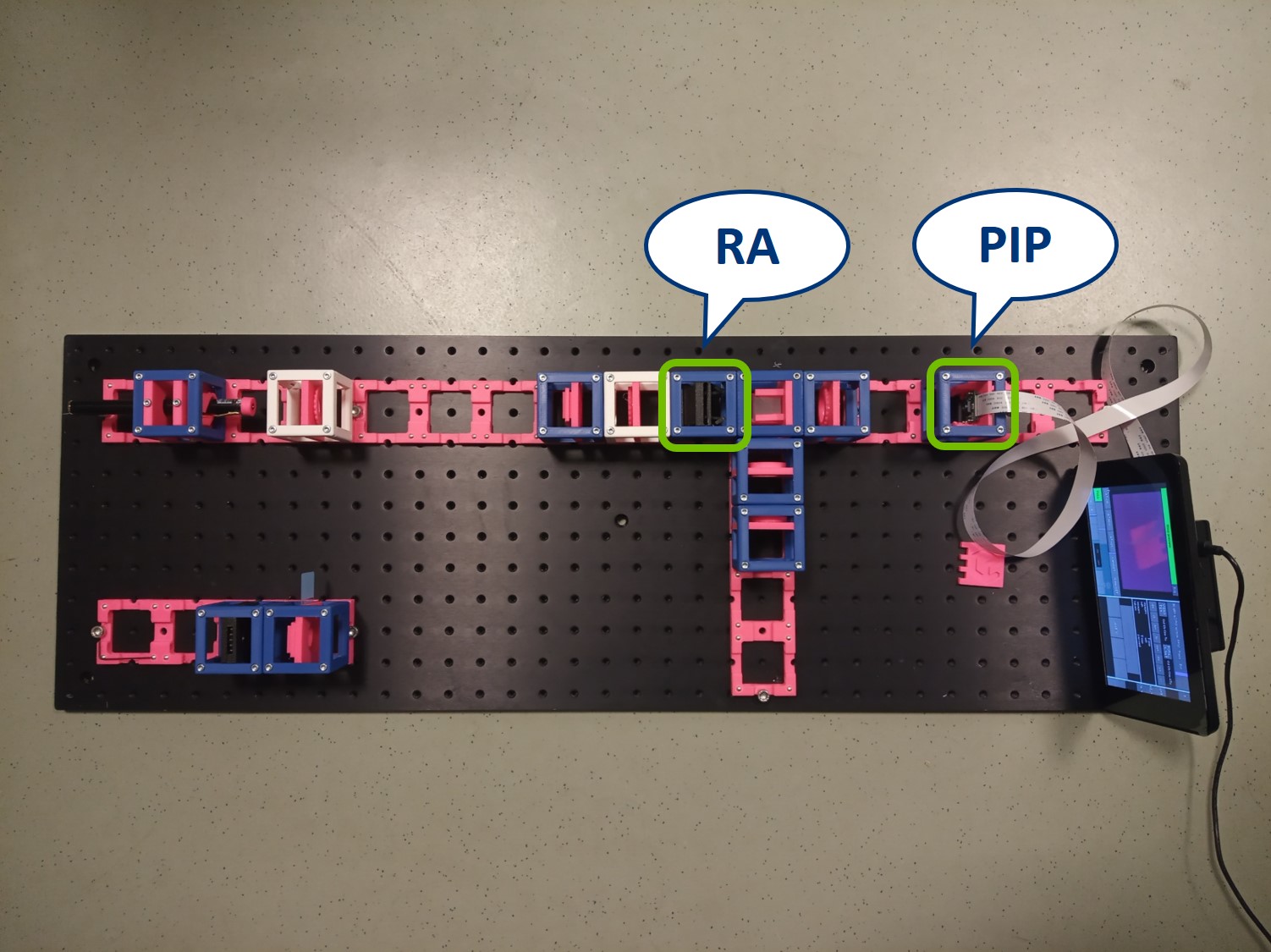
You can switch the camera between the PIP and the BFP. You could also use two cameras, one in PIP and one in BFP, if you have them.
Between the objective and the Beamsplitter is the Back Focal Plane of the Objective. You can see it if you put a piece of paper there - you will see the Fourier transform of the sample. You should see the same on camera in the side arm.
In the PIP, you can see an image of the sample. Here we see our fish net. Align the camera to obtain a sharp image.
⭐ Because of the Talbot effect you can find more than one sharp image of the sample. Therefore, partially close the Field diaphragm (FD) and find the position of the camera where you not only see a sharp image of the grating (fish net) but also of the FD.
- In the BFP image in the side arm, you can see the Fourier transform of the grating just as it looks in the BFP itself. Align the second Relay lens to obtain a focussed image on the camera.
⭐ The grating is regular in both X and Y and therefore it's a very convenient sample for this experiment, because its Fourier transform is easily predictable. With a different sample the BFP will of course also look differently.

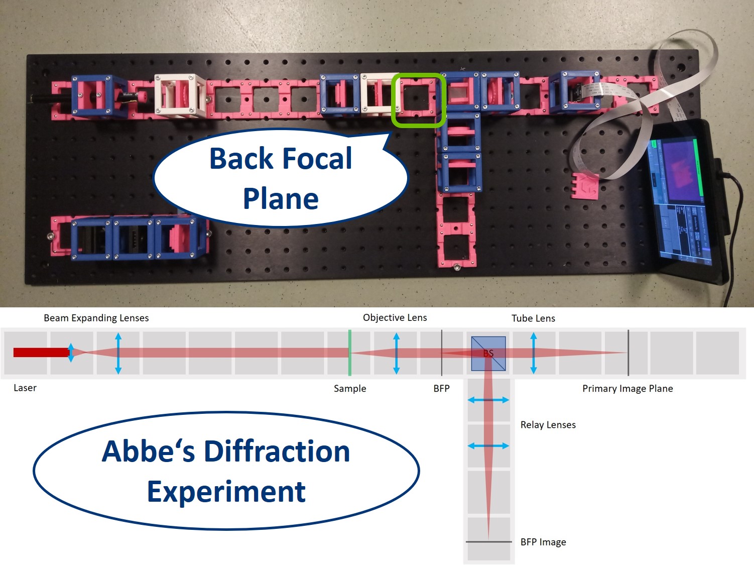
⭐ Back Focal Plane
The intensity peaks in the BFP are the diffraction orders of our sample. By placing an aperture or another object here we’ll be able to modify the information transmitted through the microscope that contributes to the image. Depending on the aperture we can observe different effects.
Circular aperture: The circular aperture blocks the light symmetrically from outside towards the center. Close the aperture and align the laser such that the 0th order is in the center of the aperture. You can align the laser using the four screws in its holder.
Rectangular aperture: The rectangular aperture closes independently from both sides in X and Y direction (horizontally and vertically). Use a hex key or a similar tool to close/open the aperture doors.
Dot and line: Use a sample holder cube or your (presumably steady) hand to hold these two. You can block the 0th or 0th+1st orders with the dot, depending on how big it is. You can block the X-0th or Y-0th order with the line-object.
- This is the setup for the second experiment: Abbe Diffraction Experiment.
⭐ Abbe Diffraction experiment - What do we see?
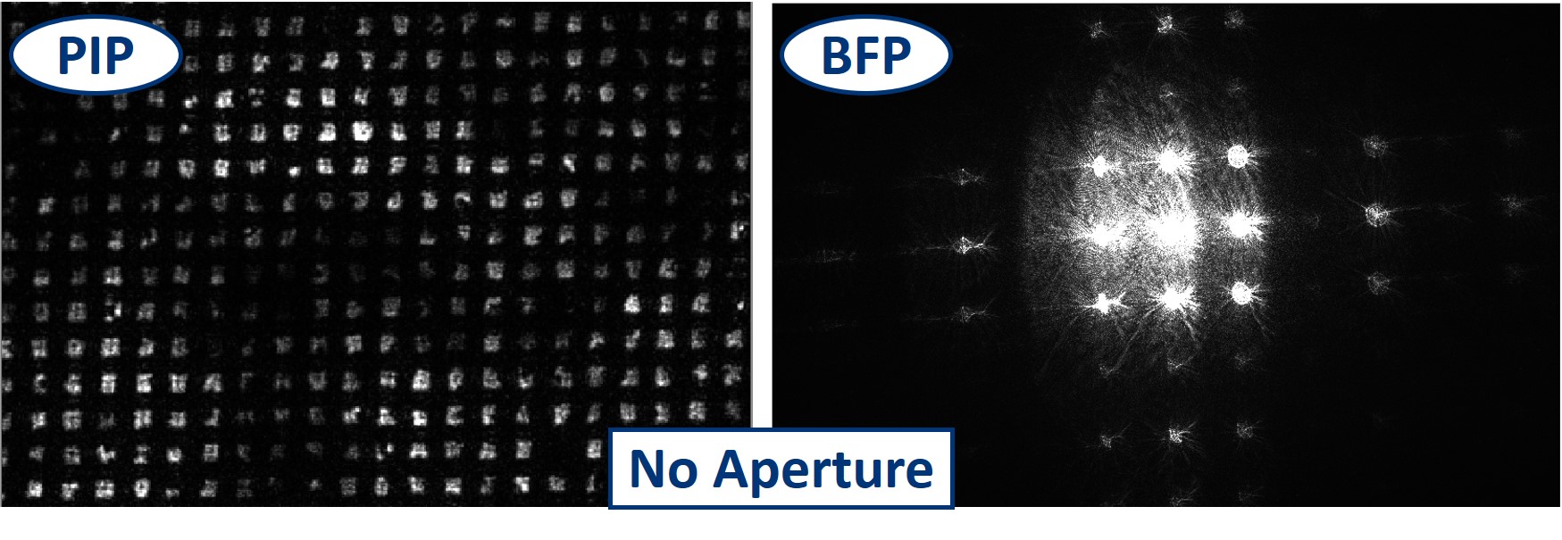
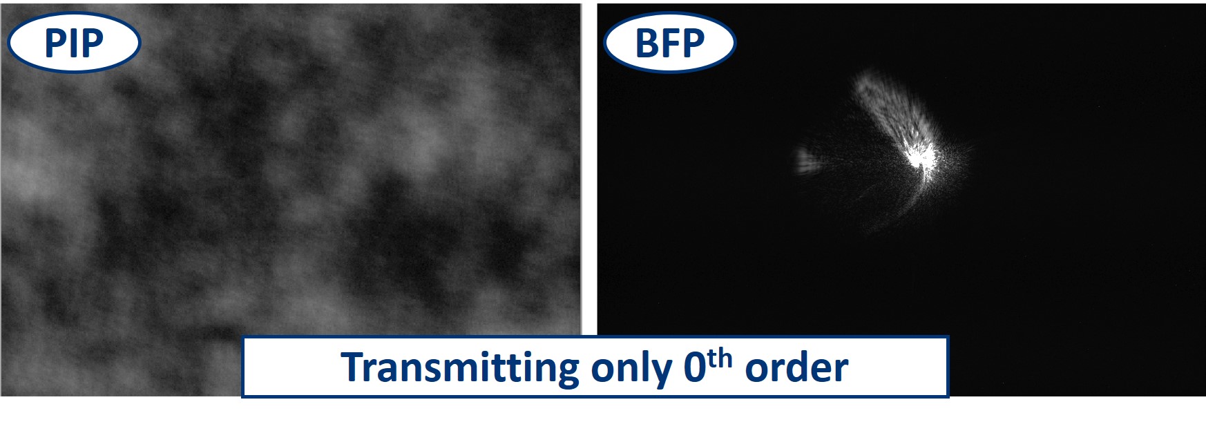
- With no aperture in the BFP, we see the image of the Sample in PIP and the Fourier transorm of the sample in the BFP, as we just aligned it and prepared it.
- Firstly we use the Circular aperture. As we slowly close it and change the diameter of the transmitting area, we cut out the higher diffraction orders that carry the high frequency information, hence the fine details. In the image plane we see how these details blur and the sharp edges soften. The more orders we cut out, the blurrier the image gets.
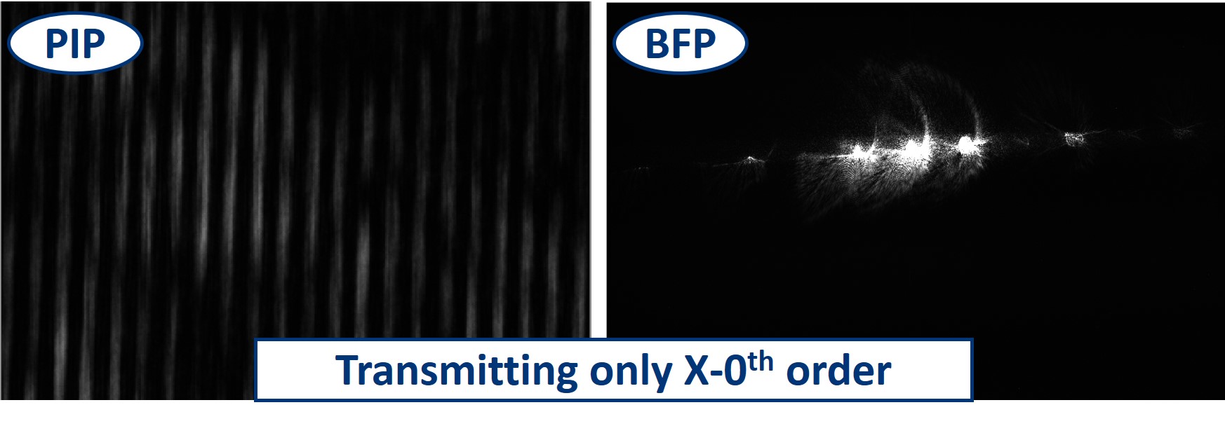
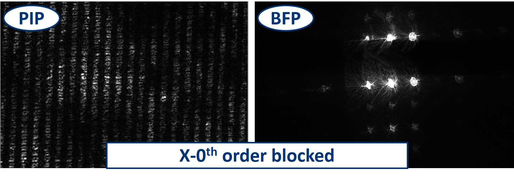
- Using the Rectangular aperture, we can block the diffraction orders more selectively. When we close the aperture in the X direction to only let through the Y-0th orders, the square pattern of the image disappears, and we have only lines. This is because there is no X order that would transmit the information about the shape in the perpendicular direction.
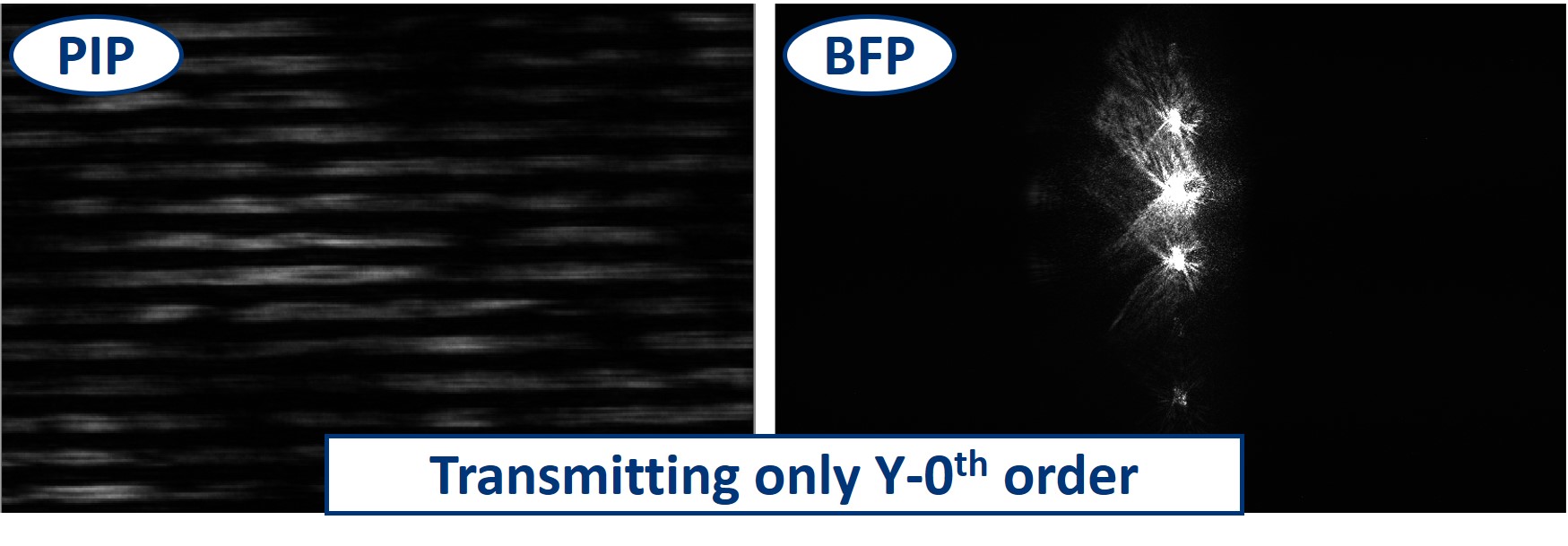
- When we do the same trick in the other direction, we then see lines of the other orientation but again no square pattern.
- Closing the aperture in both X and Y direction, we eventually block all the higher orders that form the image of the sample. As we can see here, when only the 0th order is transmitted all image information is lost. What we see is only some background noise.
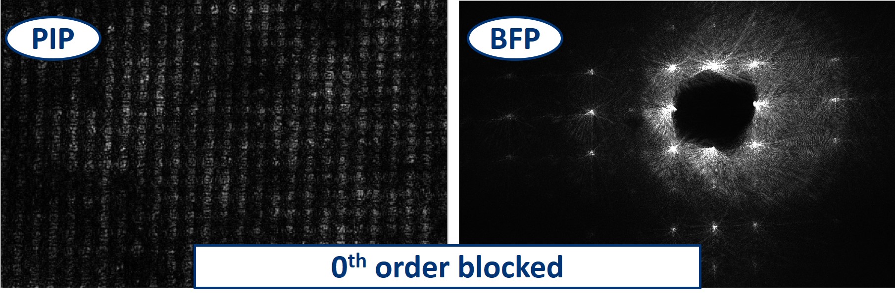
- On the other hand, when we block only the 0th order but keep all the others (we do this using the dot on a slide), we are still able to see the pattern is preserved, because all the orders still have a corresponding partner to interfere with on the other side from the 0th order. But now we are in a so-called dark field imaging mode. We'll explain it in the next steps.
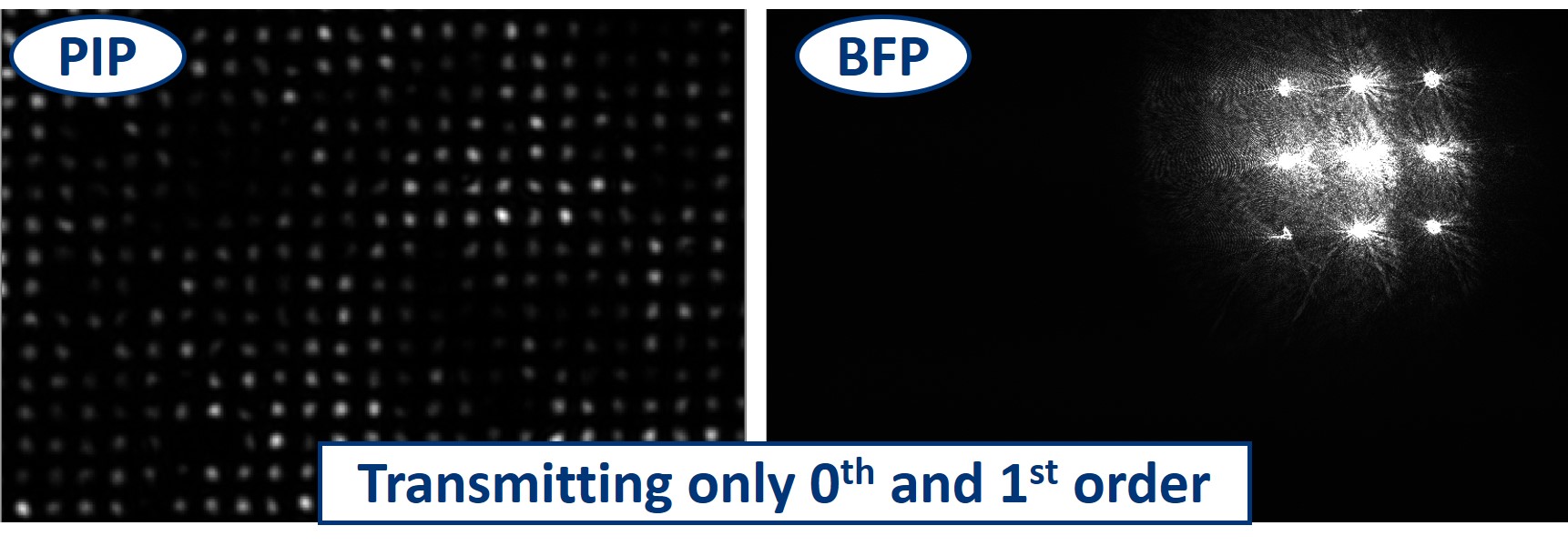
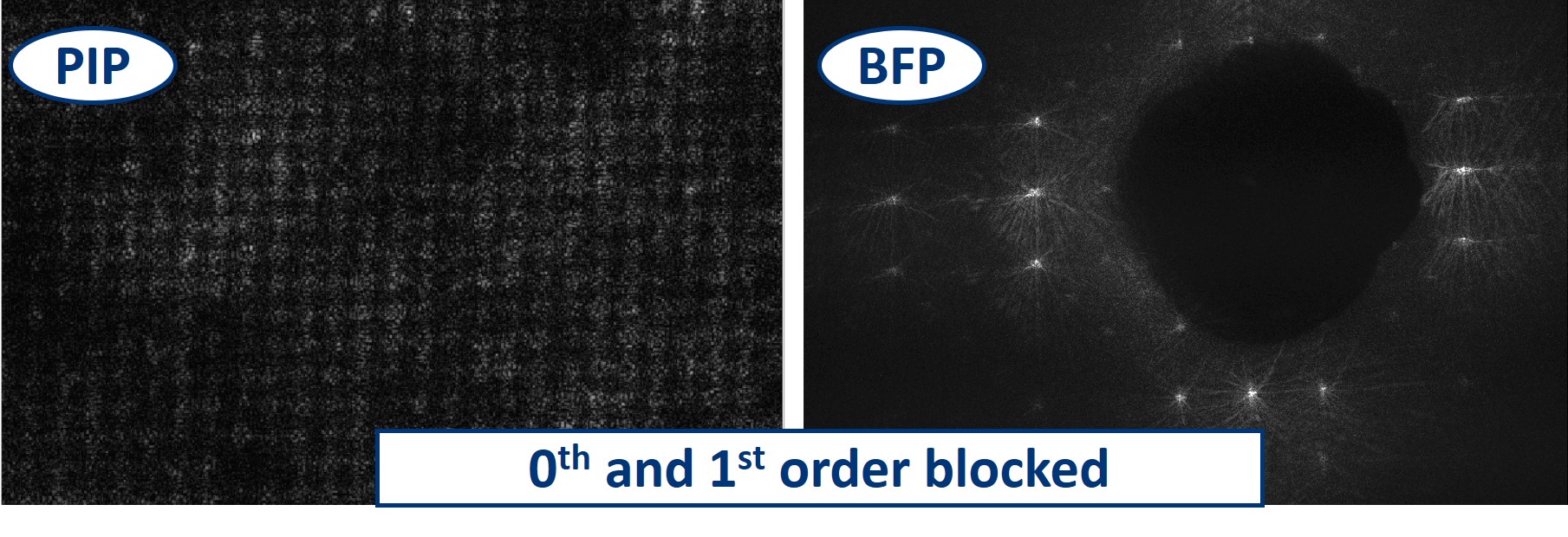
- We can even block the 0th and 1st order by simply using a bigger dot in the BFP. We are still able to recognize the square pattern but the high frequency information, the noise, is taking over the image.
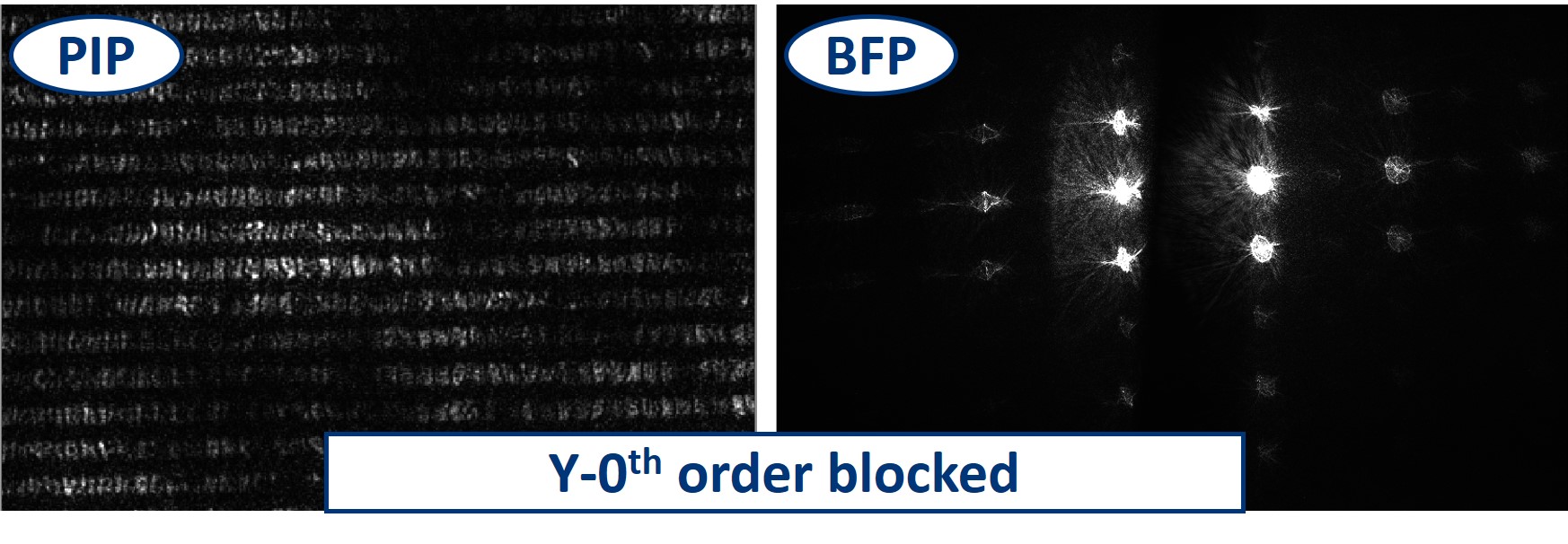
- When using the line object instead of the dot, we can block the 0th order completely in the Y direction and see what it does to the image. We still see the square pattern but suddenly, in the X direction, it seems that we have twice as many squares. This is the dark field imaging effect but in X only. We’re seeing just the edges and because there are two edges per square in one direction, it appears that we see them twice.
- The same works also in the perpendicular direction - blocking the 0th order in X results in the dark field imaging mode in Y.
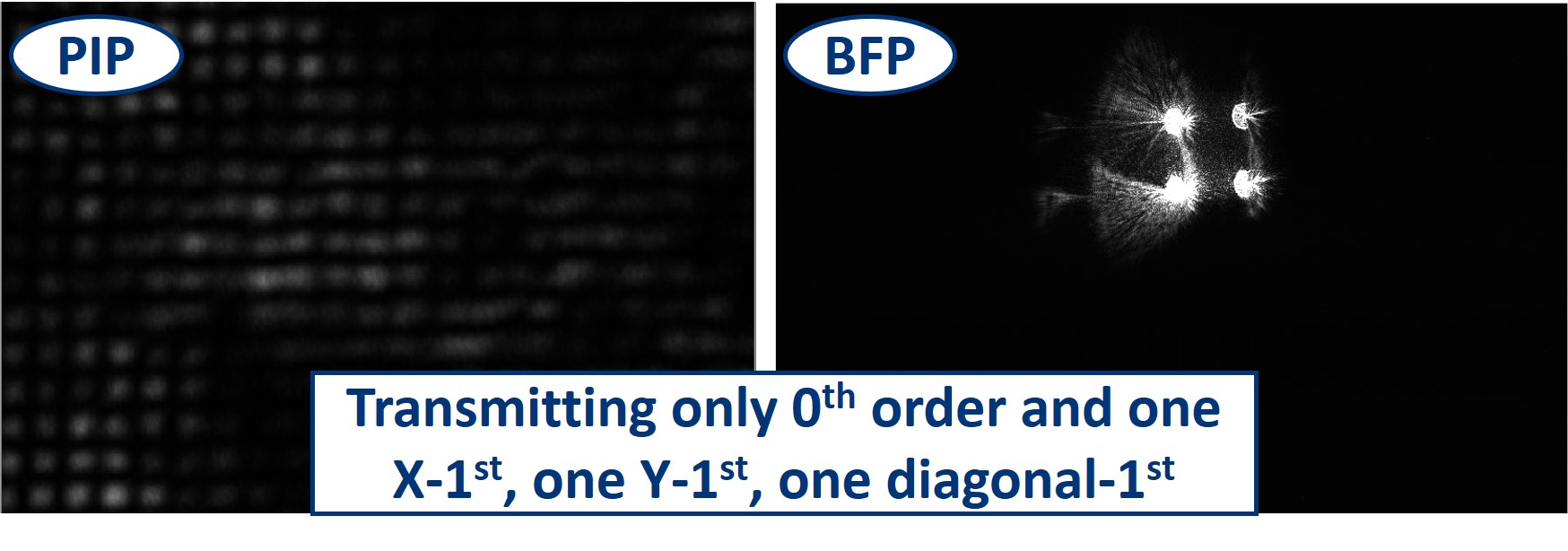
- Using the rectangular aperture again and we can find out what is the minimal amount of orders that we need to form a reliable image. We said that they always interfere with the 0th order, so we don't need both sides. Therefore, we close the aperture and let through only one quarter of the orders. We can block the higher orders as well, as they only carry the high frequency information, and we are still able to see the basic pattern of our sample.
⭐ Watch the video of this experiment!
Notes to the video:
- In this demonstration of the experiment, two Alvium cameras from Allied vision are used, so we can show the PIP and BFP on the screen simultaneously
- Find the cubes for the Alvium cameras here anch choose the adjustable insert for easy alignment.
- The optical path is different from the one described in this tutorial. This is because of the use of the above mentioned cameras
- The objective and eyepiece are both lenses with f' = 100 mm. The magnification of the microscope is therefore equal to 1. The "magnified" image is just a zoom into the camera view.
- Thanks to the use of a 10 mm lens as an objective, the diffraction orders in BFP are more separated and easily accessible.
- In the side arm, the first lens has f' = 100 mm and the second lens f' = 50 mm. The image of the BFP is therefore demagnified twice, to fit better in the field of view of the camera.
Bonus question: This magical image was taken by the RasPi camera in the BFP with the fish net as a sample. If you tell me what created this effect, I send you a chocolate ;-)

 Participate
If you have a cool idea, please don't hesitate to write us a line, we are happy to incorporate it in our design to make it even better.
References:
1; 2; 3; Cat image source;
4 Advanced Optical Imaging Workshop; Plymouth; Noah Russell, 2009©